Top Tree
Self-Adjusting Top Tree
Overview
The self-adjusting top tree (SATT) is a data structure for maintaining a fully dynamic forest. It is built on the theory of top trees and was introduced by Tarjan and Werneck in their 2005 paper Self-Adjusting Top Trees.
On any tree of the forest, a self-adjusting top tree supports path updates and queries, subtree updates and queries, non-local search, and more.
SATT is built on the splay tree, but the splay tree it uses differs from the ordinary one in some details (it is extended in a few ways).
Motivating problem
Maintain a forest under the following operations:
-
Delete or add an edge. The graph is guaranteed to be a forest before and after the operation.
-
Update the weights on a simple path of some tree.
-
Update the weights in the subtree rooted at some node.
-
Query the sum of the weights on a simple path of some tree.
-
Query the sum of the weights in the subtree rooted at some node.
Tree contraction
Any tree can be contracted to a single edge using the theory of tree contraction.
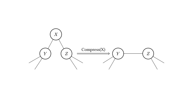
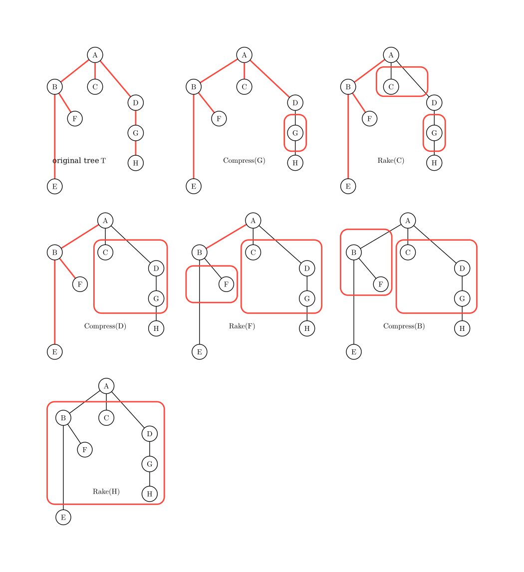
Tree contraction has two basic operations, compress and rake. Compress takes a node \(x\) of degree \(2\). Let \(y\) and \(z\) be the two nodes adjacent to \(x\). We add a new edge \(yz\), store the information of node \(x\), edge \(xz\) and edge \(xy\) in \(yz\), and delete all three, as shown.
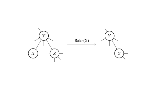
Rake takes a node \(x\) of degree \(1\) whose neighbor \(y\) has degree greater than \(1\). Let \(z\) be the other neighbor of \(y\). We store the information of node \(x\) and edge \(xy\) in edge \(yz\) and delete both, as shown.
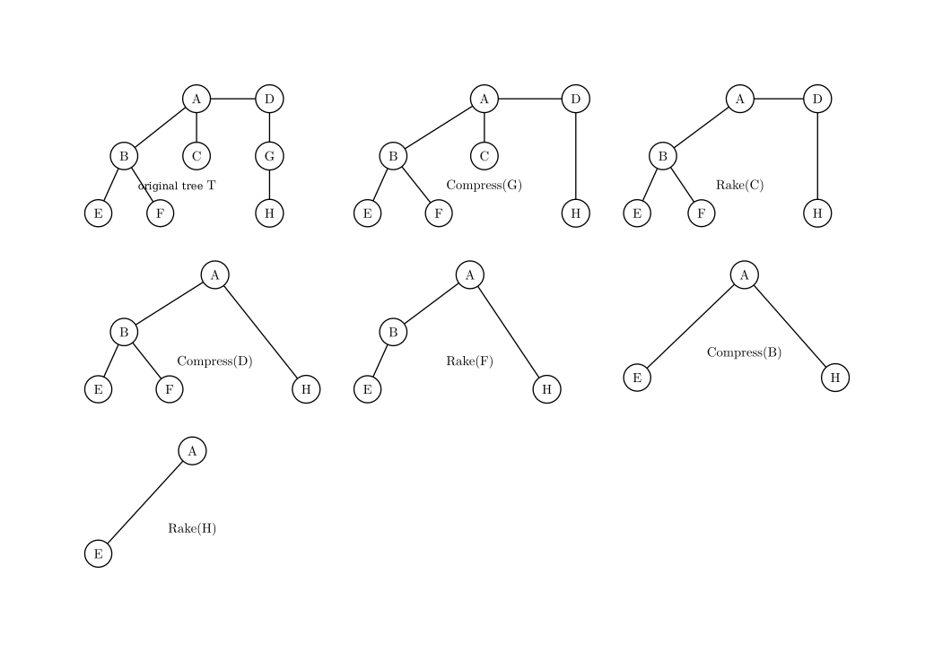
It is easy to prove that any tree can be contracted to a single edge using only compress and rake, as shown.
Clusters
For convenience, let \(T\) be the original tree before any operation, and let \(T_x\) be the tree obtained from \(T\) after some tree contraction operations (possibly none).
Let us look at what information an edge of some \(T_x\) holds.
Besides its own information (if the edge does not exist in \(T\), it has none of its own, of course), the edge may hold the information of other nodes and edges that compress and rake operations have merged into it. Pick an edge from the contraction process in the figure below and see which nodes and edges of \(T\) its information stands for.
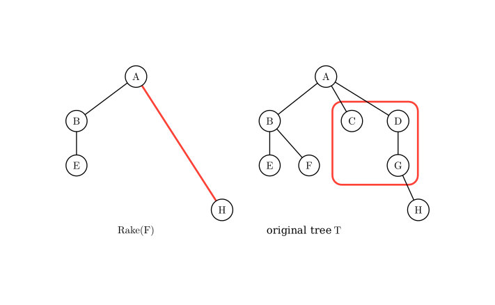
In the figure, the chosen edge and the corresponding part of the graph are circled in red.
The nodes and edges of \(T\) that this edge stands for are connected. In general, the information stored in any edge of any \(T_x\) always corresponds to a connected subgraph of \(T\). We call such a connected subgraph a cluster.
A cluster, however, is an incomplete subgraph: some of its edges have endpoints that the cluster itself does not contain. We call these the endpoints of the cluster. The nodes of the connected subgraph that it does contain are its internal nodes, and the edges of that subgraph are its internal edges.
Every cluster has the following properties:
-
A cluster stores and maintains only the information of its internal nodes and internal edges.
-
A cluster has two endpoints. They are the two nodes joined by the edge of \(T_x\) that represents the cluster. The path between the two endpoints is called the cluster path. If the endpoints of a cluster are \(x\) and \(y\), we write \(C(x,y)\) for the cluster from now on.
-
An internal node is adjacent only to endpoints and internal nodes.
In particular, every edge of \(T\) is a cluster on its own (holding only the information of the edge itself); we call such a cluster a base cluster. In the final \(T_x\), where \(T\) has been contracted to a single edge, the cluster represented by that edge holds the information of all of \(T\) except the two endpoints; we call it the root cluster.
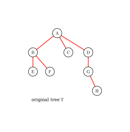
In the figure, the base clusters mentioned above are marked in red.
Seen in terms of clusters, a compress or rake operation merges two clusters into one new cluster. Tree contraction is therefore also the process of merging all base clusters into one cluster.
This gives the figure below, another way to draw a sequence of tree contraction operations.
Top Tree
We now want to represent the whole contraction process of a tree.
Either of the two representations above would do, but both are cumbersome: a contraction of \(n\) steps takes \(n\) trees to draw.
For a more compact representation of one contraction of a tree, we introduce the top tree.
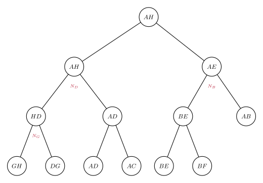
The figure shows a top tree built from the original tree and the contraction used above.
A top tree has the following properties:
-
A top tree corresponds to one original tree and one way of contracting it. Each node of the top tree represents an edge of some \(T_x\), that is, a cluster formed during the contraction. A node of the form \(N_x\) in the figure represents the cluster formed by the operation
compress(x). -
A node of a top tree has two children, each representing a cluster. The cluster of the node is the new cluster obtained by merging these two with a compress or a rake.
-
The leaves of a top tree are the base clusters and its root is the root cluster. So if we split a top tree into layers by topological order, each layer represents one \(T_x\).
Maintaining information with a ternary self-adjusting top tree
How it works
A top tree simplifies the contraction process so much that it becomes feasible to maintain information on a tree by maintaining its contraction. This is exactly how SATT works.
Tree contraction is also a process in which information on the tree is added step by step. Once we execute compress(x), the information of node \(x\) appears in some cluster from that moment on and affects our results.
Suppose we use a top tree to maintain a tree \(T\) in which every node and every edge has a weight, and what we maintain is the sum of the weights of \(T\).
Now we update the weight of some node \(x\) of \(T\). We then have to update every node of the top tree whose cluster contains \(x\), which costs \(O(n)\) per operation.
But if only a few nodes of the top tree have clusters that contain \(x\), in other words if the information of \(x\) enters a cluster as late as possible, a single operation becomes much faster. See the figure.
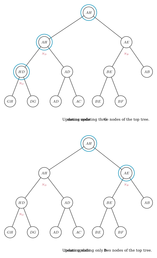
SATT maintains information on a tree by changing the order in which the information of a node or a path is added to clusters during the contraction, so that updating it becomes cheap.
The actual structure
Root the original tree \(T\), so that its nodes have depths. Now take the root cluster of the top tree of some contraction order. It has two endpoints: we require one of them to be the root of the original tree and choose the other freely.
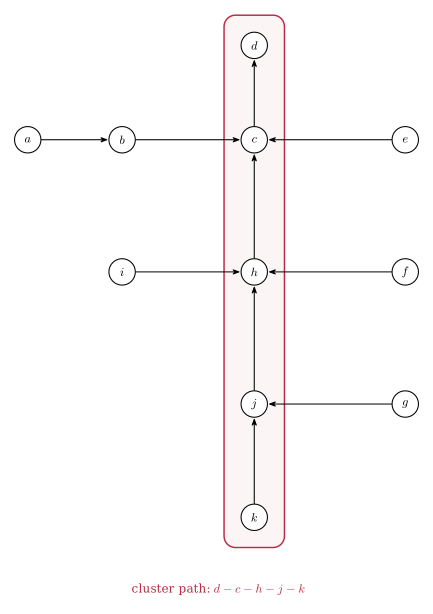
In the figure, \(d\) is chosen as the root of the original tree and \(k\) as the other endpoint of the root cluster. Arrows point from child to parent. The endpoints are drawn inside the circles that mark the clusters here.
By the basic operations of tree contraction, the nodes and edges on the cluster path, \((j,h,c,jh,hc)\), end up in \(C(k,d)\) through compress operations, whereas the nodes and edges off the cluster path, \((a,b,i,f,g,e,jg,\cdots)\), end up in \(C(k,d)\) through rake operations.
Take the cluster path out on its own. It is a tree of a special shape (a path), and we build a top tree for it (with an arbitrary contraction order).
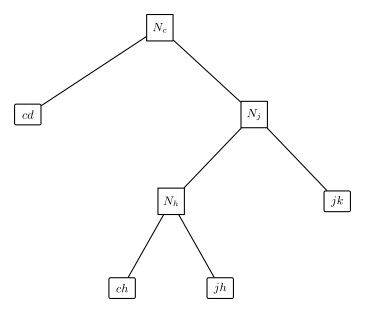
We call this structure a compress tree, because in this top tree the two children of any node merge into their parent by a compress.
The nodes of a compress tree are called compress nodes. Looking only at the current cluster path, a compress node that is not a leaf stands for one compress: it merges the information of its left and right children and then adds the information of node \(x\) that this compress(x) stores. The compress tree thus maintains the information of the cluster path of \(C(k,d)\).
Inside a compress tree we in fact restrict the top tree further. A compress tree maintains a path of \(T\) whose nodes have pairwise distinct depths. We require the inorder traversal of the base clusters in the compress tree to agree with the depths of the corresponding edges of \(T\), with earlier positions in the inorder traversal being shallower. The same holds for the nodes compress(x) and their nodes \(x\).
Now for the information off the cluster path. Suppose the nodes and edges off the cluster path have already formed maximal clusters, and that each maximal cluster is formed by raking together the smaller clusters circled in yellow. We represent the way smaller clusters merge into a maximal cluster by a ternary tree. By analogy we call this structure a rake tree, and its nodes are rake nodes. Each rake node represents a cluster, formed by raking its left and right children onto the smaller cluster represented by its middle child. As the figure below shows, the nodes of one rake tree represent smaller clusters of \(T\) that share an endpoint.
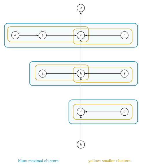
In the figure, the maximal clusters are circled in blue and the smaller clusters in yellow.
We treat the smaller clusters the same way: choose a cluster path for each, build its compress tree, and so on recursively. This produces many compress trees and rake trees that represent the contraction process.
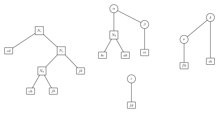
The figure above shows the rake-compress trees of the original tree (every rake node has a compress tree attached, so each looks like a rake tree with many compress trees hanging from it) and the compress tree that represents the root cluster path.
We want to join these trees so that they form one ordered whole. Let \(x\) be the common endpoint of the set of smallest clusters that a rake tree represents. To the middle child of each of these rake nodes (a set of compress trees) we add its other endpoint, the one that is not \(x\), while preserving the inorder traversal and the basic properties of a top tree, as shown.
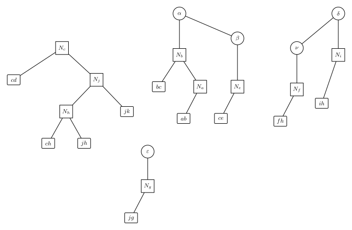
This step amounts to letting the part of a rake that adds a node of \(T\) happen inside the compress tree. Not only does this let us maintain the information of a rake node correctly (just merge the information of its three children), it also makes the structure of the compress trees more complete. Next we turn the compress tree into a ternary tree: if the common endpoint of a rake tree is \(x\), we hang that rake tree as the middle child of compress(x), as shown.
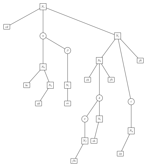
The now ternary node compress(x) means: first rake its middle child onto the cluster path, then combine the information of its left and right children and of node \(x\).
Finally we deal with the compress tree of the root cluster path. As with every other compress tree, we add its two endpoints in inorder position, so that its root stores the information of the whole of \(T\).
This is how a ternary self-adjusting top tree maintains the information of a tree.
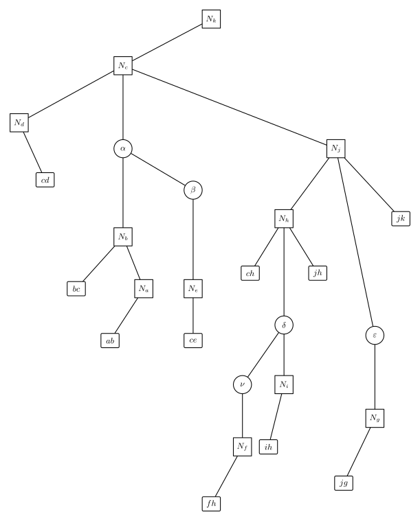
To summarize, SATT has the following properties:
-
A SATT consists of compress trees and rake trees. A compress tree is a special top tree and a rake tree is a ternary tree; both correspond to the contraction of a tree.
-
A node of a compress tree has at most three children. A compress tree can be rotated like a splay tree (it suffices to preserve its inorder traversal, and the middle child of a rotated node stays in place).
-
A node of a rake tree always has a middle child. A rake tree can be rotated like a splay tree (it suffices to preserve its inorder traversal, and the middle child of a rotated node stays in place).
-
The topological order of the SATT reflects the contraction order of the original tree \(T\).
Earlier we spoke of "changing the order in which the information of a node or a path is added to clusters during the contraction". Can SATT do this? Yes.
SATT has an operation access(x). It makes node \(x\) the non-root endpoint of the root cluster and, in the SATT, makes compress(x) the root of the SATT.
With access(x) we can rotate the node that represents compress(x) to the root of the whole SATT in amortized \(O(\log n)\). By the fourth property of SATT, this changes the position of compress(x) in the order of operations so that it is executed last, which means the information of node \(x\) is added last. To update the information of \(x\) we then only need to update compress(x).
Implementation
Push functions
Start with pulling up information, the function Pushup(x). When maintaining information at a node of the SATT, first distinguish whether the node is in a compress tree or in a rake tree; the reason was given above. As an example we maintain the subtree size of a node
1 2 3 4 5 6 7 8 9 10 11 12 | |
To query the subtree size of node \(x\), access it to the root of the SATT; the answer is the size of its middle child \(+1\). As explained above, only after the access is its middle child its proper subtree.
Next comes pushing down information, the function Pushdown(x). To update a whole subtree of the original tree, the natural idea is to access its root to the root of the SATT and put a tag on its middle child. A subtree query likewise accesses the node and queries its middle child.
To update a whole path of the original tree, expose its two endpoints. Here expose(x, y) makes node \(x\) the root of \(T\) and node \(y\) the other endpoint of the root cluster. In the SATT, the compress tree of the root cluster is then the path from \(x\) to \(y\), so we just put a tag on the compress tree of the root cluster. A path query likewise exposes the path and queries the root.
This solves the motivating problem.
1 2 3 4 5 6 7 8 9 10 11 12 13 14 15 16 17 18 19 20 21 22 23 24 25 26 27 28 29 30 31 32 | |
Splay functions
The rake trees and compress trees of a SATT can both be rotated, so they can be maintained as splay trees. This gives the following code:
1 2 3 4 5 6 7 8 9 10 11 12 13 14 15 16 17 18 19 20 21 22 23 24 25 26 27 28 29 30 31 32 | |
Note that direction and isroot differ from those of an ordinary splay tree, because the middle child of a node never changes, however the node is rotated.
Access functions
access(x) rotates node \(x\) to the root of the whole SATT and makes \(x\) one of the two endpoints of the root cluster (the other being the root of \(T\)). It must not change the structure of the original tree or its root.
To implement access(x), first rotate \(x\) to the root of its compress tree, then remove the right child of \(x\), which makes \(x\) an endpoint of the cluster of its compress tree.
1 2 3 4 5 6 7 8 9 | |
If \(x\) is now at the root, stop. Otherwise carry out the following steps to move it past the rake tree above it:
-
Splay its parent (which must be a rake node) to the root of its rake tree.
-
Splay the grandparent of \(x\) (which must be a compress node) to the root of its compress tree.
-
If the grandparent of \(x\) has a right child, swap node x with that right child, update the information, and stop.
-
If the grandparent has no right child, make \(x\) its right child. The former parent of \(x\) now has no middle child, so by the property of rake nodes above it cannot exist. Call
Deleteto remove it, and stop.
Steps 1 and 2 together are called a local splay, and steps 3 and 4 together a splice. For convenience we write them all in the function Splice(x).
The function Delete(x) mentioned above works as follows:
-
Check whether the node \(x\) to be deleted has a left child. If it does, rotate the rightmost node of the left subtree to just below \(x\) (it becomes the new left child), then make the right child of \(x\) (if any) the right child of this left child. The left child of \(x\) has now replaced \(x\). This is the merge operation of a splay tree.
-
If it has no left child, let its right child replace \(x\).
Notice that Splice(x) changes which endpoints some clusters of the original tree have. After one splice, we take the parent of \(x\) as the new \(x\) and do the next splice.
In the end, the node \(x\) we started with is the rightmost node of the compress tree of the root cluster. One final global splay rotates it to the root of the SATT.
1 2 3 4 5 6 7 8 9 10 11 12 13 14 15 16 17 18 19 20 21 22 23 24 25 26 27 28 29 30 31 32 33 34 35 36 37 38 39 40 41 42 43 44 45 46 47 48 49 50 51 52 53 54 55 56 57 58 59 60 61 62 63 64 65 66 67 68 69 70 71 | |
To make a node \(x\) the root of the original tree, access it to the root of the SATT; \(x\) is then an endpoint of the final cluster. By the inorder property of compress trees, mirroring the compress tree that contains \(x\) (swapping the left and right children of every node) makes \(x\) the root of the original tree. In the implementation we put a reversal tag on \(x\) and push it down later.
1 2 3 4 | |
expose(x, y) follows immediately:
1 2 3 4 | |
Link & Cut
Now we want to add an edge between two nodes of the original forest that are not connected. Make one of them, \(x\), the root of the original tree, and rotate the other, \(y\), to the root; \(y\) should then become the right child of \(x\). Then hang the new edge on the right child of \(y\) (in a SATT that maintains only nodes, this step can be skipped).
1 2 3 4 5 6 7 8 9 | |
Cut works much like Link
1 2 3 4 5 6 | |
Full code
Luogu P3690 [Template] Dynamic Tree
1 2 3 4 5 6 7 8 9 10 11 12 13 14 15 16 17 18 19 20 21 22 23 24 25 26 27 28 29 30 31 32 33 34 35 36 37 38 39 40 41 42 43 44 45 46 47 48 49 50 51 52 53 54 55 56 57 58 59 60 61 62 63 64 65 66 67 68 69 70 71 72 73 74 75 76 77 78 79 80 81 82 83 84 85 86 87 88 89 90 91 92 93 94 95 96 97 98 99 100 101 102 103 104 105 106 107 108 109 110 111 112 113 114 115 116 117 118 119 120 121 122 123 124 125 126 127 128 129 130 131 132 133 134 135 136 137 138 139 140 141 142 143 144 145 146 147 148 149 150 151 152 153 154 155 156 157 158 159 160 161 162 163 164 165 166 167 168 169 170 171 172 173 174 175 176 177 178 179 180 181 182 183 184 185 186 187 188 189 190 | |
Proof of the time complexity of SATT
For a SATT with \(n\) nodes in its current state \(x\), define the potential function
where \(r(i) = \lceil \log_2 \text{siz}(i) \rceil\) and \(\text{siz}(i)\) is the size of the subtree rooted at \(i\).
The amortized cost of a splay in a SATT is clearly still \(3\log n + 1\), even though a SATT is a ternary tree.
So to prove the time complexity of SATT, it suffices to prove that of the access function.
We analyze the amortized cost of an access step by step.
First we rotate node \(x\) to the root of its compress tree. The amortized cost of this step is
Then we make sure \(x\) has no right child. The amortized cost of this step is
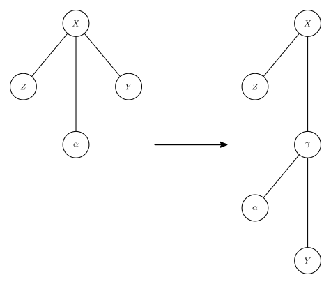
The figure shows how the right child of node \(x\) is removed.
After that, local splays and splices alternate, and after some number of splices node \(x\) has been rotated to the root of the SATT. We analyze one round of local splay and splice:
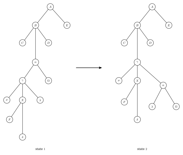
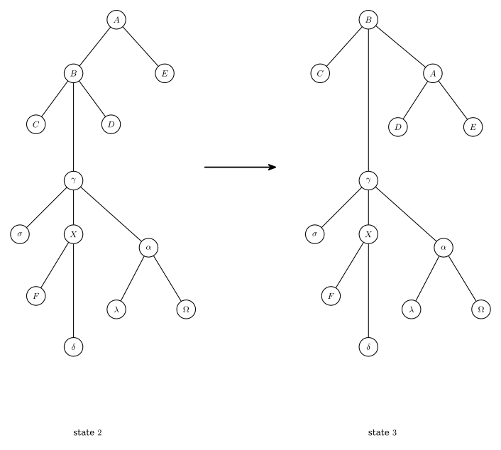
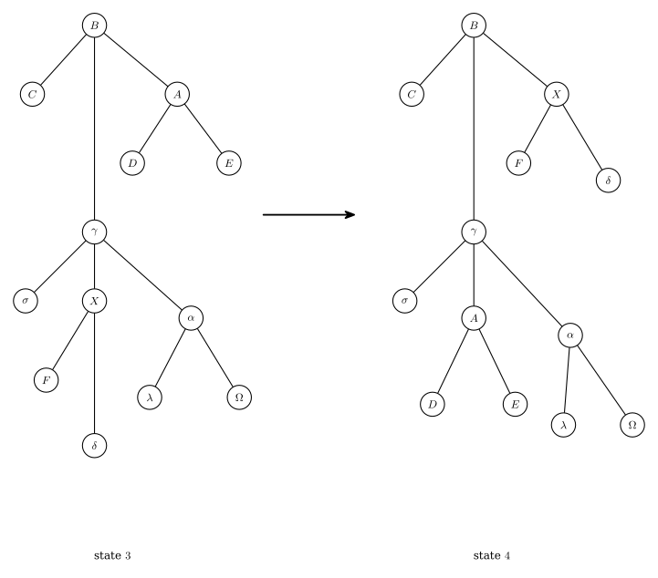
The figures show one splice on node \(x\), without the final left rotation of \(x\).
For convenience, let \(r_x(i)\) be the value of \(r\) at node \(i\) in state \(x\).
From the figures, the operation from state 1 to state 2 (the local splay that rotates the parent of node \(x\) to the root of its rake tree) has amortized cost
From the figures, the operation from state 2 to state 3 (the local splay that rotates the grandparent of node \(x\) to the root of its compress tree) has amortized cost
The operation from state 3 to state 4 (the splice) needs a closer look
Clearly \(r_4(\gamma) \leq r_3(B)\)
so the amortized cost of this operation is
Putting these together, one splice costs
Let \(r'(X)\) be the value of \(r\) at the node \(X\) of the next splice (node \(B\) in state 4). Note that \(r_3(\gamma),r_1(\gamma) \ge r_1(X)\), \(r_3(B),r_2(\gamma) \leq r'(X)\) and \(r_3(B)=r_2(B)\), so
On top of this cost, a splice may incur an extra amortized cost from delete(x); call this part \(a' \leq 3\log n +1\).
Set \(a'\) aside for now. The \(r'(X)\) of each splice equals the \(r(X)\) of the next one, and the \(r(X)\) of the first splice equals the \(r(X)\) we had when we first rotated node \(x\) to the root of its compress tree. So for the cost of one access(x), not counting delete(x), we have:
where \(k\) is the number of splices.
It looks as if the \(3k+1\) that \(a\) carries makes the amortized analysis fail, but there is a way around it. The zig-zig and zig-zag rotations can be amortized as
If we can find enough zig-zig and zig-zag operations, we can spread the \(3k+1\) over them and so get rid of it.
The global splay supplies that many zig-zig and zig-zag operations: the number of nodes in the global splay is certainly greater than \(k\), and the path from node \(x\) to the root of the global splay has no fewer than \(k\) nodes, so one access(x) contains at least \(\dfrac k2\) zig-zag operations. Adding the amortized cost \(a \leq 3\log n +1\) of the global splay, the amortized cost of one access(x), not counting delete(x), is
Now bring \(a'\) back in and write the total for \(m\) access(x) operations.
What we want is the actual cost
A delete(x) operation deletes one rake node. Over \(m\) operations we add at most \(m\) rake nodes, and by the definition of a rake node there are at most \(n\) of them initially, so in total we perform at most \(m+n\) delete(x) operations. Since \(a' \leq 3\log n +1\),
This proves the complexity of access. Every other function is either built on access or takes constant time per call, so the complexity of SATT is proved.
Incidentally, you can drop the global splay as an LCT does and instead rotate the node being accessed once at each splice; the time complexity is still correct. (In practice the version without the global splay is much faster and runs neck and neck with LCT on Luogu P3690.)
Example problems
Example 1
CEOI 2019 Dynamic Diameter
Given a tree with \(n\) nodes and edge weights, process \(q\) updates. Each update changes one edge weight and then asks for the tree diameter. Forced online.
We need a dynamic diameter. After building the SATT, maintain the answer of every node in Pushup(x) and query the answer of the root, which is the diameter of the whole tree.
1 2 3 4 5 6 7 8 9 10 11 12 13 14 15 16 17 18 19 20 21 22 | |
Here \(diam\) is the answer of the current node (the diameter of the cluster it represents) and \(len\) is the length of the cluster path of the current compress node. \(maxs_{0/1}\) is the maximum distance from the compress node to the internal nodes and endpoints of its cluster, not using its cluster-path child / not using its parent. (A rake node stores only \(maxs_0\), the maximum distance from the upper endpoint of the current cluster to the internal nodes and endpoints of the cluster.) Each query reads diam at the root of the SATT. Correctness is clear.
Pushrev(x) needs a small change.
1 2 3 4 5 6 | |
Example 2
[CSP-S 2019] Tree Centroid
Given a tree, delete each edge in turn, on its own. Each deletion splits the tree into two subtrees; take the sum of the indices of their centroids. Find the total of these sums over all edges.
If we could maintain the tree centroid dynamically in \(O(\log n)\), the problem would be solved.
SATT can maintain the tree centroid dynamically in \(O(\log n)\). Doing so requires non-local search.
A property on a tree is local if every node or edge that has it in the whole tree also has it in every subtree that contains that node or edge. Otherwise the property is non-local. Local information can usually be maintained with pushup(x)
For example, having the minimum weight is local: a node or edge whose weight is the minimum of the whole tree also has the minimum weight in every subtree that contains it. Having the second smallest weight is clearly non-local.
The \(diam\) we maintained above is also local information.
Back to the problem. The centroid is clearly non-local information and cannot be maintained by a simple pushup(x). So we search on the SATT:
The search starts from the root of the SATT, that is, from the root cluster. The centroid has a convenient property: if the number of nodes on one side of an edge is greater than or equal to the number on the other side, then that side contains at least one centroid (there may be two centroids).
Let \(sum\) be the number of nodes of a cluster, and let \(maxs\) be the maximum \(sum\) among the middle children of all rake nodes of a rake tree.
1 2 3 4 5 6 7 8 9 10 | |
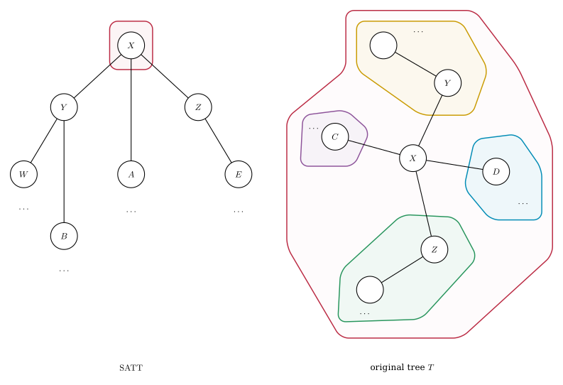
The figure shows the SATT during a non-local search and the corresponding original tree \(T\).
We make the following comparisons:
-
Compare the \(sum\) of cluster \(compress(Y)\) with the \(sum\) of the union of cluster \(compress(Z)\), cluster \(A\) and node \(X\) (call this union cluster \(\alpha\) for now). If the \(sum\) of \(compress(Y)\) is greater than or equal to the latter, at least one centroid lies in the subtree of \(compress(Y)\), and we recurse into \(compress(Y)\). (If the two are equal, node \(X\) is also a centroid and must be recorded.)
-
Compare the \(sum\) of cluster \(compress(Z)\) with the \(sum\) of the union of cluster \(compress(Y)\), cluster \(A\) and node \(X\) (call this union cluster \(\beta\) for now). If the \(sum\) of \(compress(Z)\) is greater than or equal to the latter, at least one centroid lies in the subtree of \(compress(Z)\), and we recurse into \(compress(Z)\). (If the two are equal, node \(X\) is also a centroid and must be recorded.)
-
Take the smaller cluster with the largest \(sum\) in the rake tree that is the middle child of node \(x\), and compare its \(sum\) with the \(sum\) of the union of cluster \(compress(Y)\), cluster \(A\), node \(X\) and the other smaller clusters (call this union cluster \(Y\) for now). If the \(sum\) of that smaller cluster is greater than or equal to the latter, at least one centroid lies in its subtree, and we recurse into it. If the two are equal, node \(X\) is also a centroid and must be recorded.
-
If none of the comparisons above recurses, node \(X\) is a centroid. Record it and stop.
The first step of the search is clearly correct. How should it continue?
Suppose we recurse into \(Y\). The information stored at \(Y\) is now incomplete: \(compress(Y)\) holds only the information of its own cluster, while we want the centroid of the whole tree. The fix is to carry along the information of the earlier clusters and, when comparing at node \(Y\), combine the information of the previous cluster with that of \(Y\) itself. The implementation is as follows:
1 2 3 4 5 6 7 8 9 10 11 12 13 14 15 16 17 18 19 20 21 22 23 24 25 26 27 28 29 30 31 32 33 34 35 36 37 38 39 40 41 42 43 44 45 46 47 48 49 50 51 52 53 54 55 56 57 | |
Example code
1 2 3 4 5 6 7 8 9 10 11 12 13 14 15 16 17 18 19 20 21 22 23 24 25 26 27 28 29 30 31 32 33 34 35 36 37 38 39 40 41 42 43 44 45 46 47 48 49 50 51 52 53 54 55 56 57 58 59 60 61 62 63 64 65 66 67 68 69 70 71 72 73 74 75 76 77 78 79 80 81 82 83 84 85 86 87 88 89 90 91 92 93 94 95 96 97 98 99 100 101 102 103 104 105 106 107 108 109 110 111 112 113 114 115 116 117 118 119 120 121 122 123 124 125 126 127 128 129 130 131 132 133 134 135 136 137 138 139 140 141 142 143 144 145 146 147 148 149 150 151 152 153 154 155 156 157 158 159 160 161 162 163 164 165 166 167 168 169 170 171 172 173 174 175 176 177 178 179 180 181 182 183 184 185 186 187 188 189 190 191 192 193 194 195 196 197 198 199 200 201 202 203 204 205 206 207 208 209 210 211 212 213 214 215 216 217 218 219 220 221 222 223 224 225 226 227 228 229 230 231 232 233 234 235 236 237 238 239 240 241 242 243 244 245 246 247 248 | |
Reference
-
Robert E. Tarjan and Renato F. Werneck. 2005. Self-adjusting top trees. In Proceedings of the sixteenth annual ACM-SIAM symposium on Discrete algorithms (SODA '05). Society for Industrial and Applied Mathematics, USA, 813–822. DOI 10.5555/1070432.1070547
-
negiizhao's blog (in Chinese)
This page is an unofficial English translation of the original OI Wiki page (revision 9bb3a8e6), machine-translated by Claude Fable 5.2 on 2026-11-16. It has been modified from the original by translation and may contain errors. It is not endorsed by OI Wiki.
Found a translation problem? Report it on GitHub.
Authors of the original page: F7487, hsfzLZH1, 24OI-bot, Enter-tainer, AtomAlpaca, liuzimingc, HeRaNO, Tiphereth-A, not-exist, sun2snow (full contribution history)
All content on this page is provided under the terms of CC BY-SA 4.0 and SATA; additional terms may apply.