Block-Cut Tree
Before reading this page, make sure you know the material in Graph Theory Concepts.
Further reading: Articulation Points and Bridges.
Introduction
As is well known, trees (and forests) have nice properties and are easy to maintain with many common data structures.
General graphs are not so well behaved. Fortunately, some problems on a general graph can be moved to a tree.
The block-cut tree (also called the block forest or round-square tree)1 is one way to turn a graph into a tree. This article covers how to build it, its properties and some applications.
For reasons of space, some results in this article are stated without proof; work them out or prove them yourself.
Definition
The block-cut tree started out as a tool for cactus graphs (undirected graphs in which every edge lies on at most one simple cycle). Once more of its properties are brought out, though, it can sometimes be used on general undirected graphs.
To introduce the block-cut tree, we first need biconnected components.
One definition of a biconnected graph is: any two distinct vertices are joined by at least two vertex-disjoint paths.
Vertex-disjoint means both that no path repeats a vertex (each is a simple path) and that the two paths have an empty intersection (apart from the start and end vertices, of course, which both paths necessarily pass through).
For a graph with a single vertex it is hard to say whether it is biconnected, so for now we leave aside graphs with \(1\) vertex.
An almost equivalent definition is: a graph with no articulation point.
This definition breaks down only for the graph that consists of two vertices and one edge joining them. That graph has no articulation point, yet it does not contain two disjoint paths, because it has only one path.
(You can also take the view that this one path counts twice; the two copies are indeed disjoint, since the path passes through no other vertex.)
The first definition is the original one, but for convenience we adopt the second.
A biconnected component of a graph is then a maximal biconnected subgraph.
Unlike with strongly connected components and the like, a vertex may belong to several biconnected components, but every edge belongs to exactly one (under the first definition, an edge might belong to none).
In the block-cut tree, every vertex of the original graph corresponds to a round node and every biconnected component to a square node.
So the tree has \(n+c\) nodes in total, where \(n\) is the number of vertices of the original graph and \(c\) is the number of its biconnected components.
The square node of each biconnected component is joined by an edge to every vertex of that component.
Each biconnected component thus forms a star graph, and the stars are joined to one another at the articulation points of the original graph (because the vertices that separate biconnected components are articulation points).
Clearly, every edge of the block-cut tree joins a round node and a square node.
The figures below show a graph, its biconnected components and the shape of its block-cut tree.2
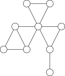
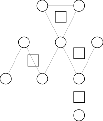
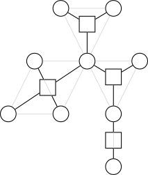
The block-cut tree has fewer than \(2n\) nodes, because there are fewer than \(n\) articulation points, so remember to make every array twice as large.
Strictly speaking, the block-cut tree is a tree only if the original graph is connected. If the original graph has \(k\) connected components, its block-cut tree is a forest of \(k\) trees.
A connected component of the original graph that consists of a single vertex has to be handled case by case; the rest of this article ignores isolated vertices.
Procedure
How do we construct the block-cut tree of a graph? If the graph is disconnected, each connected component can be handled separately, so we consider only connected graphs.
The block-cut tree is built on biconnected components, which are in turn built on articulation points, so a method much like the one for finding articulation points is all we need.
Articulation points are usually found with Tarjan's algorithm. If you know it, what follows will be easy; if you don't, that is fine too.
We skip Tarjan's algorithm for articulation points and go straight to the algorithm used for the block-cut tree (which is really a variant of Tarjan's):
Run a DFS on the graph. It relies on two key arrays, dfn and low (much as Tarjan's algorithm does).
dfn[u] stores the DFS order of node \(u\), that is, the position of \(u\) in the order in which the nodes are first visited.
low[u] stores the smallest DFS order of a node that some node \(v\) in the subtree of \(u\) in the DFS tree can reach through at most one back edge or tree edge to its parent.
This may be hard to follow if you have never heard of Tarjan's algorithm, so let us look at an example:
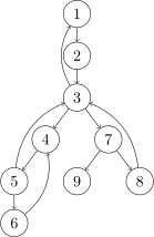
(This graph is in fact equivalent to the one in the figures above.)
Tree edges are drawn here as straight lines going downward, and back edges as curves going upward. The label of a node is its DFS order.
The low array is then:
| \(i\) | \(1\) | \(2\) | \(3\) | \(4\) | \(5\) | \(6\) | \(7\) | \(8\) | \(9\) |
|---|---|---|---|---|---|---|---|---|---|
| \(\mathrm{low}[i]\) | \(1\) | \(1\) | \(1\) | \(3\) | \(3\) | \(4\) | \(3\) | \(3\) | \(7\) |
Not too hard, is it? Note that the low of \(9\) is \(7\) here, which differs from some ways of finding articulation points: for convenience, we allow going up through the edge to the parent. The main idea is the same.
The DFS function that computes dfn and low is easy to write (the dfn array is all zeros initially):
Implementation
1 2 3 4 5 6 7 8 9 10 | |
1 2 3 4 5 6 7 8 9 10 | |
Next we look at how biconnected components relate to the DFS tree and to these two arrays.
Each biconnected component is a connected subtree of the DFS tree and contains at least two nodes; in particular, its topmost node has exactly one node of the component directly below it.
Every tree edge also lies in exactly one biconnected component.
Take the topmost node \(u\) of a biconnected component in the DFS tree. We identify the component at \(u\), because the subtree of \(u\) holds all the information about it.
The component has at least two nodes, so take its next node \(v\); there is a tree edge between \(u\) and \(v\).
In this situation \(\mathrm{low}[v]=\mathrm{dfn}[u]\) must hold.
More precisely, for a tree edge \(u\to v\), the nodes \(u\) and \(v\) lie in the same biconnected component and \(u\) is the node of smallest depth in that component if and only if \(\mathrm{low}[v]=\mathrm{dfn}[u]\).
So during the DFS we can tell where a biconnected component is, but not yet exactly which nodes it contains.
This is not hard to deal with: during the DFS, maintain a stack of the nodes whose biconnected component (or components, since there may be several) has not been determined yet.
When a biconnected component is found, all of its nodes other than \(u\) sit together at the top of the stack, so we just keep popping until \(v\) has been popped.
The popped nodes can of course be processed on the spot: add an edge between each of them and the newly created square node. At the end, add an edge between \(u\) and the square node as well.
This builds the block-cut tree quite naturally. Label the square nodes with integers starting from \(n+1\), which makes round nodes and square nodes easy to tell apart.
This part may not have been explained clearly enough, so here is the code, with detailed comments, print statements that help you follow it, and a sample. Copy the code and try it out yourself; after all, nothing helps understanding as much as code (don't forget to enable c++11).
Implementation
1 2 3 4 5 6 7 8 9 10 11 12 13 14 15 16 17 18 19 20 21 22 23 24 25 26 27 28 29 30 31 32 33 34 35 36 37 38 39 40 41 42 43 44 45 46 47 48 49 50 51 52 53 54 55 56 57 58 59 | |
Here is a test case:
1 2 3 4 5 6 7 8 9 10 11 12 13 14 15 16 | |
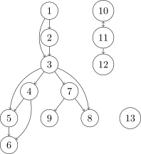
The graph for this example (it includes a multiple edge and an isolated vertex):
Example problems
Here are some example problems that can be solved with a block-cut tree.
[APIO2018] Duathlon
Problem summary
Given a simple undirected graph, count the triples \(\langle s, c, f \rangle\) (\(s, c, f\) pairwise distinct) for which there is a simple path that starts at \(s\), passes through \(c\) and ends at \(f\).
Solution
Simple paths call for a very nice property of biconnected components: for two vertices of a biconnected component, the union of the simple paths between them is exactly that component.
In other words, between two distinct vertices \(u,v\) of a biconnected component there is always a simple path that passes through any given third vertex \(w\) of the same component.
Proof of this property:
- Clearly a simple path that leaves a biconnected component can never come back to it, as that would contradict the definition of a biconnected component.
- So it suffices to prove that for any three distinct vertices \(u,v,c\) of a biconnected graph, there is a simple path from \(u\) to \(v\) that passes through \(c\).
- First set aside the graph with \(2\) vertices: it has the property, but you cannot pick \(3\) distinct vertices in it.
- For the remaining cases, build a network flow model: add an edge of capacity \(2\) from the source to \(c\), and an edge of capacity \(1\) from each of \(u\) and \(v\) to the sink.
- Each undirected edge \(\langle x,y\rangle\) of the original graph becomes an edge of capacity \(1\) from \(x\) to \(y\) and another edge of capacity \(1\) from \(y\) to \(x\).
- Finally, give every vertex other than the source, the sink and \(c\) a capacity of \(1\), which can be done by vertex splitting.
- The edge from the source to \(c\) has capacity \(2\), so if the maximum flow of this network is \(2\), there must be a path that passes through \(c\).
- Apply the max-flow min-cut theorem: the minimum cut is clearly at most \(2\), so it remains to prove that it is greater than \(1\).
- This is equivalent to proving that cutting any one edge of capacity \(1\) cannot disconnect the source from the sink.
- Suppose we cut the edge that joins \(u\) or \(v\) to the sink. By the first definition of biconnectivity, there is a simple path from \(c\) to the other one, whose edge has not been cut.
- Suppose we cut the edge created by splitting a vertex. This amounts to deleting a vertex, and by the second definition of biconnectivity the rest of the graph is still connected.
- Suppose we cut an edge built from an edge of the original graph. This amounts to deleting an edge, which is weaker than deleting a vertex, so a path clearly exists.
- So the minimum cut is greater than \(1\), that is, the maximum flow equals \(2\). This completes the proof.
What does this result tell us? Take the path between two round nodes in the block-cut tree: the set of round nodes adjacent to the square nodes on that path is exactly the set of vertices on the simple paths between the two vertices in the original graph.
Back to the problem. Fix \(s\) and \(f\) and count the valid \(c\): clearly this count is the number of vertices in the union of the simple paths between \(s\) and \(f\), minus \(2\) (to exclude \(s\) and \(f\) themselves).
So once the block-cut tree of the original graph is built, the number of vertices on the simple paths between two vertices depends on the number of square nodes (biconnected components) and round nodes on their path in the block-cut tree.
Now for a common block-cut tree trick: when aggregating over paths, give the nodes suitable weights.
In this problem, each square node gets the size of its biconnected component as its weight, and each round node gets weight \(-1\).
With these weights, the sum of the node weights on the block-cut tree path between two round nodes is exactly the size of the union of the simple paths in the original graph, minus \(2\).
The problem becomes computing, in the block-cut tree, \(\sum\) of the path weight sums over pairs of round nodes.
Look at it from the other side: count each node's contribution to the answer, which is its weight times the number of paths through it. A simple tree DP computes this.
Finally, don't forget the case where the graph is disconnected. The code follows:
Reference code
1 2 3 4 5 6 7 8 9 10 11 12 13 14 15 16 17 18 19 20 21 22 23 24 25 26 27 28 29 30 31 32 33 34 35 36 37 38 39 40 41 42 43 44 45 46 47 48 49 50 51 52 53 54 55 56 57 58 59 60 61 62 63 64 65 66 67 68 69 70 71 72 73 74 75 76 77 | |
Incidentally, the answer to this problem for the test case above is \(212\).
Codeforces #487 E. Tourists
Problem summary
Given a simple connected undirected graph, support two operations:
-
Update the weight of a vertex.
-
Query the minimum vertex weight on all simple paths between two vertices.
Solution
Again we build the block-cut tree of the original graph. Let the weight of a square node be the minimum weight of its adjacent round nodes; the problem becomes a path minimum query.
Path minima can be maintained with heavy-light decomposition and a segment tree. But what about updates?
Updating the weight of one round node means updating every square node adjacent to it, and adversarial data can easily force \(O(n)\) such updates.
Here we use the fact that the block-cut tree is a tree: let the weight of a square node be the minimum weight among its own child round nodes. An update then only has to touch the parent square node.
To maintain the square nodes, keep a multiset of weights for each of them.
Note that if the LCA in a query is a square node, the weight of the LCA's parent round node has to be checked as well.
Note: allocate twice as many nodes for the block-cut tree as the original graph has; otherwise you get an out-of-bounds array access.
Reference code
1 2 3 4 5 6 7 8 9 10 11 12 13 14 15 16 17 18 19 20 21 22 23 24 25 26 27 28 29 30 31 32 33 34 35 36 37 38 39 40 41 42 43 44 45 46 47 48 49 50 51 52 53 54 55 56 57 58 59 60 61 62 63 64 65 66 67 68 69 70 71 72 73 74 75 76 77 78 79 80 81 82 83 84 85 86 87 88 89 90 91 92 93 94 95 96 97 98 99 100 101 102 103 104 105 106 107 108 109 110 111 112 113 114 115 116 117 118 119 120 121 122 123 124 125 126 127 128 129 130 131 132 133 134 135 136 137 138 139 140 141 142 143 144 | |
[SDOI2018] Strategy Game
Problem summary
You are given a simple connected undirected graph and \(q\) queries:
Each query gives a vertex set \(S\) (\(2 \le |S| \le n\)) and asks for the number of vertices \(u\) with \(u \notin S\) whose deletion leaves the vertices of \(S\) no longer all in one connected component.
Each test contains multiple test cases.
Solution
Build the block-cut tree first. A query then asks for the number of round nodes in the connected subgraph of the block-cut tree that corresponds to \(S\), minus \(|S|\).
How do we count the round nodes in this connected subgraph? Here is one way:
Move the weight of each round node onto the edge between it and its parent square node. The problem becomes a sum of edge weights; for that, see one of the solutions to [SDOI2015] Treasure Hunt Game.
That is, sort the nodes of \(S\) by DFS order and add up the distances between consecutive nodes in the sorted order (including the distance between the first and the last). The answer is half of this sum of distances, because every edge is traversed exactly twice.
Finally, if the shallowest node of the subgraph is a round node, add \(1\) to the answer, because it has not been counted.
There are multiple test cases, so remember to initialize the arrays.
Reference code
1 2 3 4 5 6 7 8 9 10 11 12 13 14 15 16 17 18 19 20 21 22 23 24 25 26 27 28 29 30 31 32 33 34 35 36 37 38 39 40 41 42 43 44 45 46 47 48 49 50 51 52 53 54 55 56 57 58 59 60 61 62 63 64 65 66 67 68 69 70 71 72 73 74 75 76 77 78 79 80 81 82 83 84 85 86 87 88 89 90 91 92 93 94 | |
Practice problems
- UVa 1464 Traffic Real Time Query
- Luogu P4320 Encounter on the Road
- Luogu P10517 National Land Planning
External links
immortalCO, The Round-Square Tree: A Powerful Tool for Cacti (in Chinese), Universal OJ.
References and notes
-
In 2017, Junkun Chen defined this structure and named it the round-square tree in his IOI2017 Chinese national training team paper Problem-Setting Report on "Magical Subgraph" and Its Extensions (in Chinese). ↩
-
Junkun Chen, The Ordinary Round-Square Tree and the Magical (
Dynamic) Dynamic Programming (in Chinese), NOI2018 Winter Camp, p. 4. ↩
This page is an unofficial English translation of the original OI Wiki page (revision 9bb3a8e6), machine-translated by Claude Fable 5.2 on 2026-11-16. It has been modified from the original by translation and may contain errors. It is not endorsed by OI Wiki.
Found a translation problem? Report it on GitHub.
Authors of the original page: GitPinkRabbit, Early0v0, Backl1ght, mcendu, ksyx, iamtwz, Xeonacid, kenlig, Menci, Enter-tainer, CCXXXI, hcx2012Git, StudyingFather, 24OI-bot, shawlleyw, scp020, Tiphereth-A, c-forrest, Plastic-time (full contribution history)
All content on this page is provided under the terms of CC BY-SA 4.0 and SATA; additional terms may apply.