Divide and Conquer on Trees
Centroid decomposition
Centroid decomposition works well for problems about paths in large trees.
Example 1: Luogu P3806 [Template] Centroid Decomposition 1
Given a tree with \(n\) nodes and edge weights, answer \(m\) queries. Each query gives \(k\) and asks whether the tree contains a pair of nodes at distance \(k\).
\(n\le 10000,m\le 100,k\le 10000000\)
Pick an arbitrary node \(\mathit{rt}\) as the root. The paths that lie entirely inside its subtree are of two kinds: those that pass through the current root and those that do not. The paths through the root are again of two kinds: those that have the root as an endpoint, and those whose endpoints are both different from the root. A path of the second kind can be obtained by combining two paths of the first kind. So for each root \(rt\) that we enumerate, we first compute the contribution to the answer of the paths in its subtree that pass through it, and then recurse into its child subtrees to handle the paths that do not.
In this problem, we handle the paths through the root \(\mathit{rt}\) as follows. Enumerate the children \(\mathit{ch}\) of the root and, with \(\mathit{ch}\) as the root of its subtree, compute the distance from every node in the subtree of \(\mathit{ch}\) to \(\mathit{rt}\). Let \(\mathit{dist}_i\) be the distance from node \(i\) to the current root \(rt\), and let \(\mathit{tf}_{d}\) say whether one of the subtrees processed so far contains a node \(v\) with \(\mathit{dist}_v=d\). If the \(k\) of a query satisfies \(tf_{k-\mathit{dist}_i}=true\), then a path of length \(k\) exists. Once we have checked whether the paths into the subtree of \(\mathit{ch}\) give an answer, we add the new distances to the array \(\mathit{tf}\).
Do not clear the array \(\mathit{tf}\) with memset. Instead, put every position of \(\mathit{tf}\) that has been used into a queue and clear exactly those positions; otherwise the time bound is lost.
In centroid decomposition, all the recursive calls on one level together process each node once. If the recursion has \(h\) levels, the total running time is \(O(hn)\).
If we always choose the centroid of the subtree as the root, the recursion has the fewest levels and the running time is \(O(n\log n)\). This choice is what gives the technique its name, centroid decomposition of a tree.
After choosing a new root, always recompute the subtree sizes. Otherwise a change that looks tiny can make the time complexity wrong or the correctness hard to guarantee.
Reference code
1 2 3 4 5 6 7 8 9 10 11 12 13 14 15 16 17 18 19 20 21 22 23 24 25 26 27 28 29 30 31 32 33 34 35 36 37 38 39 40 41 42 43 44 45 46 47 48 49 50 51 52 53 54 55 56 57 58 59 60 61 62 63 64 65 66 67 68 69 70 71 | |
Example 2: Luogu P4178 Tree
Given a weighted tree with \(n\) nodes and a number \(k\), count the pairs of nodes in the tree at distance at most \(k\).
\(n\le 40000,k\le 20000,w_i\le 1000\)
Here we count the pairs of nodes whose distance lies in \([0,k]\), so we use a segment tree to maintain the distances and answer the queries.
Reference code
1 2 3 4 5 6 7 8 9 10 11 12 13 14 15 16 17 18 19 20 21 22 23 24 25 26 27 28 29 30 31 32 33 34 35 36 37 38 39 40 41 42 43 44 45 46 47 48 49 50 51 52 53 54 55 56 57 58 59 60 61 62 63 64 65 66 67 68 69 70 71 72 73 74 75 76 77 78 79 80 81 82 83 84 85 86 87 88 89 90 91 92 93 94 95 96 97 98 99 100 101 102 103 104 105 106 107 108 109 110 111 112 113 114 115 116 117 118 119 120 121 122 123 124 125 126 127 128 129 130 131 132 133 134 135 | |
Example 3: Luogu P2664 A Game on a Tree
Every node of a tree has a color. Define \(s(i,j)\) as the number of colors on the path from \(\mathit{i}\) to \(\mathit{j}\), and \(\mathit{sum_{i}}=\sum_{j=1}^n s(i,j)\). Find \(sum_i\) for every \(1\leq i\leq n\). (\(1 \le n, c_i \le 10^5\))
This problem is a real test of how well you understand the idea of centroid decomposition and can apply it. It makes a good harder example and exercise for the technique.
The first step is a change of viewpoint. The problem defines \(\mathit{sum_i}\) as the sum, over all nodes, of the number of colors on the path from \(i\) to that node. Counting it that way is awkward in centroid decomposition, because it is hard to combine the information of two subtrees that hang from the current root. So we give \(\mathit{sum_i}\) a different meaning. For each color \(j\), let \(\mathit{cnt_j}\) be the number of paths that have \(i\) as an endpoint and contain color \(j\); then \(\mathit{sum_i}\) is just \(\sum \mathit{cnt_j}\). All this does is change what we look at: we now consider the contribution of each color to \(\mathit{sum_i}\). And \(\mathit{cnt_j}\) is easy to compute: every time we meet a new color, do \(\mathit{cnt_{col_u}}+=\mathit{size_u}\), where \(\mathit{size_u}\) is the size of the subtree of u, because every node of that subtree contributes one to the answer of \(u\) for this color.
In centroid decomposition we then only need to count two things separately:
- what the paths in the subtree that have the current root as an endpoint contribute to the root;
- what the paths whose LCA is the current root contribute to each node of the subtree.
Part 1 is easy. The recursion in centroid decomposition has at most \(\log{n}\) levels, so on every level we can afford to traverse the whole subtree, and we count with the definition of \(\mathit{sum_i}\) along the way.
For part 2, let \(d\) be a child of the current root \(u\), and let \(v\) be any node in the subtree of \(d\). The answer of \(v\) splits into two parts:
- Colors that occur on the path \((u, v)\). Let \(\mathit{num}\) be their number, and let \(\mathit{siz1}\) be the total size of all subtrees of \(u\) other than that of \(d\). These colors contribute \(\mathit{num}\times \mathit{siz1}\) to the answer of \(v\).
- Colors \(j\) that do not occur on the path \((u, v)\). Their contribution comes from the \(\mathit{cnt_j}\) of all subtrees of \(u\) other than that of \(d\), and this part of the answer is \(\sum_{j \notin (u, v)} \mathit{cnt_j}\).
That is the whole counting idea. See the reference code for the implementation details.
Reference code
1 2 3 4 5 6 7 8 9 10 11 12 13 14 15 16 17 18 19 20 21 22 23 24 25 26 27 28 29 30 31 32 33 34 35 36 37 38 39 40 41 42 43 44 45 46 47 48 49 50 51 52 53 54 55 56 57 58 59 60 61 62 63 64 65 66 67 68 69 70 71 72 73 74 75 76 77 78 79 80 81 82 83 84 85 86 87 88 89 90 91 92 93 94 95 96 97 98 99 100 101 102 103 104 105 106 107 108 109 110 111 112 113 114 115 116 117 118 119 120 121 122 123 124 125 126 127 128 129 130 131 132 133 134 135 136 137 138 139 140 141 142 143 144 | |
Edge centroid decomposition
As in centroid decomposition above, we pick an edge that splits the tree into two parts as evenly as possible (the \(\mathit{size}\) of the two subtrees that the edge joins should be as close as possible). Then we recurse into the left and right subtrees and collect the information.
But this does not work. Consider a star graph:
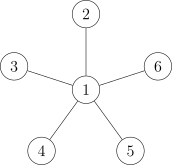
When a node has many children of similar \(\mathit{size}\), edge centroid decomposition is unacceptably slow.
If the graph is a binary tree, the weakness that the star graph exposes disappears. So we turn a multiway tree into a binary tree.
Clearly, it is enough to build the tree the way a segment tree is built, like this:
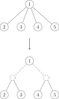
Give the newly created nodes whatever information the problem calls for. For example, when counting path lengths, set the weight of every original edge to \(1\) and the weight of every new edge to \(0\).
As for the complexity: at most \(O(n)\) nodes are added, so the total complexity is \(O(n\log n)\).
Almost every centroid decomposition problem can also be solved by edge centroid decomposition (the constant factor differs, but not by enough to fail the time limit), so we give no example problems here.
Centroid tree
A centroid tree is a tree rebuilt from the original tree: the shape of the tree is changed so that its number of levels is always \(\log n\).
It is commonly used for problems with updates that do not depend on the shape of the original tree.
Analysis of the algorithm
We rebuild the original tree by repeatedly finding centroids, exactly as centroid decomposition does.
Make every centroid we find a child of the centroid of the level above. This gives a tree with \(\log n\) levels.
Because the tree has \(\log n\) levels, many brute-force approaches that would be too slow on the original tree have the right complexity on the centroid tree.
Implementation
A small trick: take the total size \(\mathit{tot}\) of the previous level of the recursion and subtract the size of the heavy child of the previous level's node. The result is the total size of the current level, so finding the centroid takes only one DFS.
Reference code
1 2 3 4 5 6 7 8 9 10 11 12 13 14 15 16 17 18 19 20 21 22 23 24 25 26 27 28 29 30 31 32 33 34 35 36 37 38 39 40 41 42 43 44 45 46 47 48 49 50 51 52 53 54 55 56 57 58 59 60 61 62 63 64 65 66 67 68 69 70 71 72 73 74 75 76 77 78 79 80 | |
This page is an unofficial English translation of the original OI Wiki page (revision 9bb3a8e6), machine-translated by Claude Fable 5.2 on 2026-11-16. It has been modified from the original by translation and may contain errors. It is not endorsed by OI Wiki.
Found a translation problem? Report it on GitHub.
Authors of the original page: Ir1d, hsfzLZH1, Marcythm, Xeonacid, partychicken, 24OI-bot, ouuan, Henry-ZHR, Chrogeek, StudyingFather, thallium, Enter-tainer, ksyx, mcendu, fanfansann, kenlig, chenyanlann, shuzhouliu-bot, Early0v0, Konano, Alphnia, shuzhouliu, zirnc, Tiphereth-A, r-value, alphagocc, megakite, c-forrest (full contribution history)
All content on this page is provided under the terms of CC BY-SA 4.0 and SATA; additional terms may apply.