Slope Trick
Introduction
Consider a two-dimensional DP whose value function \(f(i,x)\) is convex in \(x\) for every fixed \(i\). Treating the whole function \(f(i,\cdot)\) as the state at \(i\), and maintaining its differences (or slopes)
instead of the function itself, often speeds up the transitions. This way of optimizing a DP is called the slope trick.
The term "slope"
Most functions in these problems are defined only at integer points, so it makes no real difference whether we call this quantity a difference or a slope. Following the name of the technique, this article calls it a slope throughout.
How the slopes are maintained varies from problem to problem. When the slopes lie in a narrow range, it is easier to maintain the points where the slope changes (the breakpoints); when the domain of the function is small, it may be easier to maintain the sequence of slopes itself. Harder cases may need both the slope and the length of every linear piece. Whatever the representation, the idea is the same: a transition changes the sequence of slopes only a little, and this is what makes the transition simple. All of these techniques count as the slope trick.
Convex functions
Before turning to problems, we need the basic properties of convex functions and how their slopes change under various transformations.
Convex functions on the real line
The general definition of a convex function is stated on \(\mathbf R\).
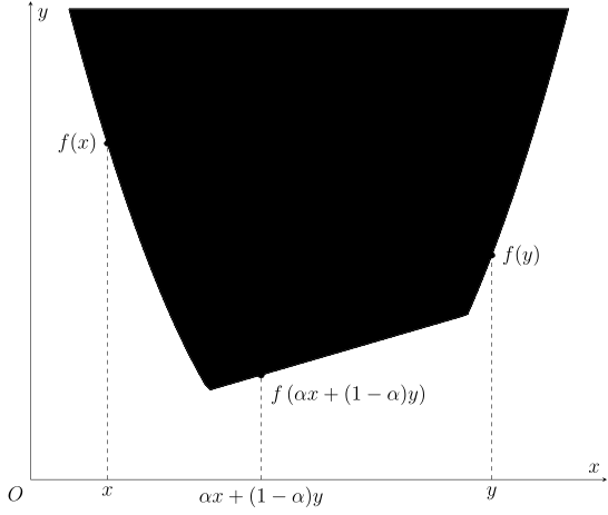
Convex functions on \(\mathbf R\)
A function \(f:\mathbf R\rightarrow\mathbf R\cup\{\pm\infty\}\) that satisfies, for all \(x,y\in\mathbf R\) and \(\alpha\in(0,1)\),
is called a convex function. The rules for \(\pm\infty\) are that \(\pm\infty\) times any positive real, or plus any real, is itself, and that \(-\infty<x<+\infty\) for every real \(x\in\mathbf R\).
If the inequality is reversed to \(\ge\), the function is called concave1. Since \(-f\) is convex whenever \(f\) is concave, this section considers convex functions only.
This article considers proper convex functions only
To avoid assigning a value to \(\infty-\infty\) and the extra analysis that comes with it, we always assume that a convex function never takes the value \(-\infty\) and is not identically \(+\infty\). Such a function is called a proper convex function. This is enough for everything that comes up in competitive programming.
A function \(f\) is often not defined for all reals. If the domain of \(f\) is only a subset of \(\mathbf R\), extend \(f\) to a function on \(\mathbf R\):
We then call \(f\) convex if and only if the corresponding \(\tilde f\) satisfies the definition above. So, unless stated otherwise, every convex function in this article has the real numbers \(\mathbf R\) as its domain. Clearly a convex function \(f\) can take finite values only on an interval (that is, on a convex subset of \(\mathbf R\)).
Simple examples
Common examples of convex functions include:
- constant functions: \(f(x)=c\) with \(c\in\mathbf R\);
- linear functions: \(f(x)=kx+b\) with \(k,b\in\mathbf R\) and \(k\neq 0\);
- absolute value functions: \(f(x)=|x-a|\) with \(a\in\mathbf R\);
- the restriction of any convex function to an interval, for example \(0_{[a,b]}(x)\) (which convex analysis calls the indicator function of \([a,b]\)).
More complicated convex functions can be built from these with the convexity-preserving transformations described below.
Convex functions on a discrete set
In competitive programming many functions are defined only at some of the integers. In general they are not convex functions in the sense above, because their domain is no longer a convex set. To cover this case, convexity has to be defined separately for functions on a discrete set. In short: first extend the domain of the function to an interval by linear interpolation, then ask whether the result is convex.
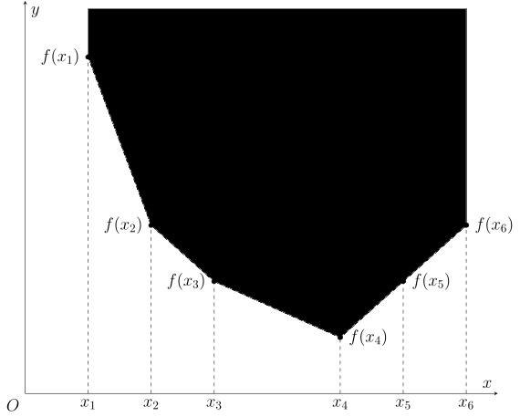
Convex functions on a discrete set
Let \(S\subset\mathbf R\) be a discrete set, that is, \(S\cap[a,b]\) is finite for every closed interval \([a,b]\). For a function \(f:S\rightarrow\mathbf R\cup\{\pm\infty\}\), define a function \(\tilde f:\mathbf R\rightarrow\mathbf R\cup\{\pm\infty\}\) as follows:
- if \(x\in S\), then \(\tilde f(x)=f(x)\);
-
if \(x\in(\inf S,\sup S)\setminus S\), let \(s_-=\max\{s\in S:s\le x\}\) and \(s_+=\min\{s\in S:s\ge x\}\), and set
\[ \tilde f(x) = \dfrac{s_+-x}{s_+-s_-}f(s_-)+\dfrac{x-s_-}{s_+-s_-}f(s_+), \] -
if \(x\notin[\inf S,\sup S]\), then \(\tilde f(x)=+\infty\).
If \(\tilde f(x)\) is a convex function on \(\mathbf R\), then \(f(x)\) is called a convex function on \(S\).
Convex functions on \(\mathbf R\) are easier to work with, so unless stated otherwise a convex function in this article means a convex function on \(\mathbf R\). When a function is given only at some of the integers, its values at the other reals are those of \(\tilde f\) in the definition; in effect we discuss the corresponding piecewise linear function \(\tilde f\) directly.
Convex functions on the integers \(\mathbf Z\) have a more intuitive equivalent definition:
Equivalent definition of convex functions on \(\mathbf Z\)
A function \(f:\mathbf Z\rightarrow\mathbf R\cup\{\pm\infty\}\) is convex if and only if
holds for all \(x\in\mathbf Z\).
Proof
This is an easy corollary of the slope characterization of convex functions.
If \(f\) is a convex function on \(\mathbf Z\), then, since its slopes are weakly increasing,
This is exactly the condition above.
Conversely, suppose the condition holds. For any \(x_1<x_2\) we have
This is the arithmetic mean of the differences over all \(i\) with \(x_1\le i<x_2\). Increasing \(x_2\) by one inserts a larger difference; increasing \(x_1\) by one removes the smallest difference. Either way the mean weakly increases. Hence the slope \(\Delta f(x_1,x_2)\) is weakly increasing, that is, \(f\) is a convex function on \(\mathbf Z\).
In other words, any sequence whose slopes (differences) are non-decreasing can be regarded as a convex function on \(\mathbf Z\).
Two characterizations of convex functions
The characterization by slopes extends to the general case.
Slope characterization of convex functions
Let \(S\) be \(\mathbf R\) or a discrete subset of it. A function \(f:S\rightarrow\mathbf R\cup\{\pm\infty\}\) is convex if and only if the slope
is a weakly increasing function of both \(x_1\) and \(x_2\) over all \(x_1,x_2\in S\) with \(x_1<x_2\).
Proof
Take a function \(f(x)\) on \(\mathbf R\), points \(x_1<x_2\) and \(\alpha\in(0,1)\), and let \(x_3=\alpha x_1+(1-\alpha)x_2\). Then
is equivalent to
Each of these two inequalities is equivalent to \(f(x_3)\le\alpha f(x_1)+(1-\alpha)f(x_2)\), which is the convexity of \(f(x)\).
Now take a function \(f(x)\) on a discrete subset \(S\) of \(\mathbf R\). That weakly increasing slopes are necessary follows from the convexity of \(\tilde f(x)\). For sufficiency, it is enough to show that \(\Delta\tilde f(x_1,x_2)\) is weakly increasing too. Write \(S=\{s_i\}\) with \(s_i\) strictly increasing in \(i\), and let \(s_{i_1}\le x_1\le s_{i_1+1}\) and \(s_{i_2}\le x_2\le s_{i_2+1}\), so that \(i_1\le i_2\). With \(\Delta_i=\Delta f(s_i,s_{i+1})\), we claim that \(\Delta_{i_1}\le\Delta\tilde f(x_1,x_2)\le\Delta_{i_2}\).
There are two cases. If \(i_1=i_2\), then \(\Delta_{i_1}=\Delta\tilde f(x_1,x_2)=\Delta_{i_2}\) and the inequality holds trivially. Otherwise,
The slopes on \(S\) are increasing, so \(\Delta_i\) is increasing in \(i\), and therefore \(\Delta_{i_1}\le\Delta\tilde f(x_1,x_2)\le\Delta_{i_2}\).
Now apply this claim. For \(x_1<x_2\) and \(\alpha\in(0,1)\), let \(x_3=\alpha x_1+(1-\alpha)x_2\) and choose \(i_3\) such that \(s_{i_3}\le x_3\le s_{i_3+1}\). Then
Substituting the expression for \(x_3\) gives the convexity of \(\tilde f(x)\).
Non-decreasing slopes can therefore serve as an equivalent definition of a convex function. Because the slopes of a convex function are monotonic, they are usually maintained in a data structure such as a heap (priority queue) or a balanced tree.
This article also uses another equivalent characterization of convex functions. For a function \(f:\mathbf R\rightarrow\mathbf R\cup\{\pm\infty\}\), consider the region of the plane that lies on or above its graph:
This region is called the epigraph of \(f\). A function is convex exactly when its epigraph is:
Epigraph characterization of convex functions
A function \(f:\mathbf R\rightarrow\mathbf R\cup\{\pm\infty\}\) is convex if and only if \(\operatorname{epi}f\) is a convex set in \(\mathbf R^2\).
Proof
If \(f\) is convex, then for \((x_1,y_1),(x_2,y_2)\in\operatorname{epi}f\) and any \(\alpha\in(0,1)\),
Hence \(\alpha(x_1,y_1)+(1-\alpha)(x_2,y_2)\in\operatorname{epi}f\).
Conversely, if \(\operatorname{epi}f\) is a convex set, then for any \(x_1<x_2\) and \(\alpha\in(0,1)\),
This is equivalent to \(\alpha f(x_1)+(1-\alpha)f(x_2)\ge f\left(\alpha x_1+(1-\alpha)x_2\right)\), which is the convexity of \(f\).
As we will see shortly, the epigraph connects the infimal convolution of convex functions with the Minkowski sum of convex sets.
Transformations of convex functions
Next we describe the convexity-preserving transformations that come up most often in the slope trick.
Nonnegative linear combinations
For convex functions \(f\) and \(g\) and nonnegative reals \(\alpha,\beta\ge0\), the function \(\alpha f+\beta g\) is convex as well. Moreover,
So if we maintain the slopes of the convex functions \(f\) and \(g\), the slopes of their nonnegative linear combination \(\alpha f+\beta g\) can be computed piece by piece.
In problems that maintain slopes, one of the two functions usually has a simple form, and a lazy tag then makes the update cheaper. In problems that maintain breakpoints, the breakpoints of \(f+g\) are obtained by merging the breakpoints of \(f\) and \(g\).
Infimal convolution (Minkowski sum)
Another common operation on convex functions is infimal convolution. For functions \(f\) and \(g\), the function
is called the infimal convolution2 of \(f\) and \(g\). If \(f\) and \(g\) are both convex, so is their infimal convolution.
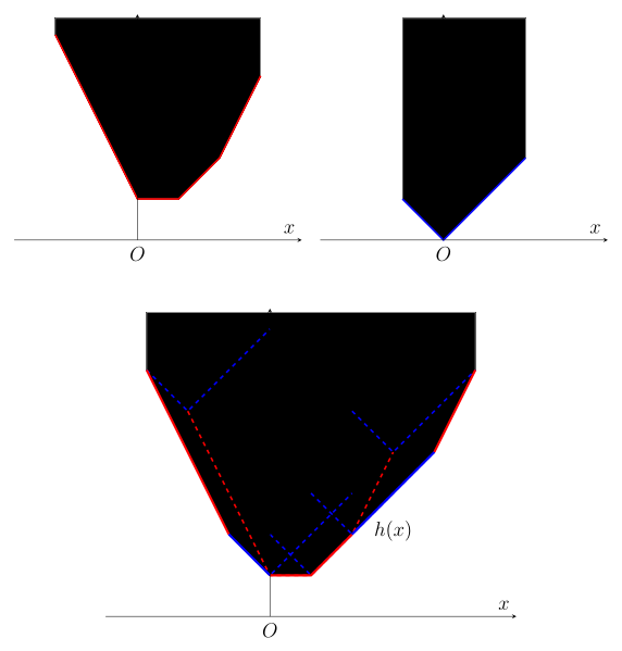
Explanation of the figure
As the figure shows, to find the infimal convolution \(h\) of \(f\) and \(g\) we can treat every point on the graph of \(f\) (the red dashed line in the third panel) as an origin and draw the graph of \(g\) in the corresponding coordinate system (the blue dashed lines in the third panel). As the origin slides along the graph of \(f\), the graph (epigraph) of \(g\) sweeps out a region, and the outline of that region, its lower hull, is the graph of \(h\). Every linear piece of \(h\) is a piece of either \(f\) or \(g\); the pieces have merely been re-sorted by slope. The roles of \(f\) and \(g\) can be swapped: sliding the graph of \(f\) along the graph of \(g\) gives the same result.
Geometrically, \(\operatorname{epi}h\) is the Minkowski sum of \(\operatorname{epi}f\) and \(\operatorname{epi}g\). If \(f\) and \(g\) are both piecewise linear functions, then so is \(h\), and its pieces are the pieces of \(f\) and \(g\) merged (and then sorted).
Proof
Let \(f\) and \(g\) be convex functions and \(h\) their infimal convolution. Let \(x_1<x_2\) and \(\alpha\in(0,1)\). By the definition of infimal convolution, for every \(\varepsilon>0\) there exist \(y_i,z_i\in\mathbf R\) with \(y_i+z_i=x_i\) and
Combining the convexity of \(f\) and \(g\) with the definition of \(h\), we get
Since \(\varepsilon>0\) was arbitrary,
So \(h\) is convex.
As for the geometric picture, strictly speaking only the following can be proved:
Here \(\operatorname{cl}\) denotes the closure.
For any \((x,y)\in\operatorname{epi} f + \operatorname{epi} g\) there exist \((x_1,y_1)\in\operatorname{epi} f\) and \((x_2,y_2)\in\operatorname{epi} g\) such that \(x=x_1+x_2\) and
Hence \((x,y)\in\operatorname{epi}h\), which shows that \(\operatorname{epi} f + \operatorname{epi} g\subseteq \operatorname{epi}h\).
Conversely, any \((x,y)\in\operatorname{epi}h\) satisfies \(y\ge h(x)\). By the definition of \(h\), for every \(\varepsilon>0\) there exist \(x_1+x_2=x\) such that
Let \(y_1=f(x_1)\) and \(y_2=g(x_2)\); then \(y+\varepsilon>y_1+y_2\). So for every \(\varepsilon>0\) there is a point \((x_1,y_1)+(x_2,y_2)\in\operatorname{epi} f + \operatorname{epi} g\) on the segment joining the points \((x,y)\) and \((x,y+\varepsilon)\). Letting \(\varepsilon\rightarrow 0\) gives \(\operatorname{epi}h \subseteq \operatorname{cl}(\operatorname{epi} f + \operatorname{epi} g)\).
So \(\operatorname{epi} f + \operatorname{epi} g = \operatorname{epi}h\) whenever \(\operatorname{epi} f + \operatorname{epi} g\) is a closed set. One condition that guarantees this is that \(f\) and \(g\) are both proper convex functions and lower semicontinuous. This is enough for the applications in competitive programming: piecewise linear functions, for example, always satisfy these conditions.
In practice, if one of \(f\) and \(g\) has only a few pieces, insert them directly among the pieces of the other. Otherwise you may need small-to-large merging, a mergeable heap or a similar method to bring down the total cost of merging, or an approach tailored to the problem.
Taking a minimum or maximum
The maximum of two convex functions is again convex, but the minimum of two convex functions need not be.
Many common minimum operations can be rewritten as infimal convolutions:
Examples
-
\(f(x)=\min_{y\in [x+a,x+b]}g(y)\) is still convex, because it is an infimal convolution:
\[ f(x) = \min_{y\in\mathbf R}g(y) + 0_{[-b,-a]}(x-y). \] -
\(f(x)=\min\{g(x-a_i)+b_i\}\) is a convex function on \(\mathbf Z\), provided that \(g(x)\) is a convex function on \(\mathbf Z\) and the function \(h:a_i\mapsto b_i\), defined on the finite set \(\{a_i\}\subset\mathbf Z\), is convex on that discrete set. The reason is that the extended function \(\tilde f(x)\) is an infimal convolution:
\[ \tilde f(x) = \min_{y\in\mathbf R}\tilde h(y)+\tilde g(x-y). \]Hence the function \(f(x)\) before the extension is convex as well.
But not every minimum operation preserves convexity.
Counterexample
Let \(g(x)\) be a convex function. The function \(f(x)=\min\{g(x-1)+kx,g(x)\}\) is not necessarily convex.
In some special problems, the dynamic programming recurrence is a minimum of two convex functions that is hard to rewrite as an infimal convolution, and yet the value function stays convex. In practice, how the slopes should change in such a problem usually has to be found by precomputing a table of values and guessing.
With convex functions and their common transformations in hand, we can see on concrete problems how the slope trick optimizes a DP. The examples in this article fall roughly into two groups, maintaining breakpoints and maintaining slopes, and show the usual operations and implementation details of each representation. As stressed earlier, though, the representation is not the essence of the slope trick: choose whichever way of maintaining the linear pieces suits the problem.
Maintaining breakpoints
Problems of this kind usually ask you to minimize a sum of several absolute values. The slopes of the value function are then small in absolute value, so it is easier to maintain the breakpoints where the slope changes.
Maintaining breakpoints means maintaining the points of a piecewise linear function at which the slope changes. For each piece \([l_i,r_i]\) of slope \(k_i\) we store only its endpoints and not the slope itself; so in these problems the slope must change by the same fixed amount every time it changes. For example, maintaining the set of breakpoints \(\xi_{-s}\le\cdots\le\xi_{-1}\le\xi_{1}\le\cdots\le\xi_{t}\) means the following: the slope is \(0\) on the interval \([\xi_{-1},\xi_1]\); it decreases by one at every breakpoint we pass going left and increases by one at every breakpoint we pass going right. So the slope is \(2\) on the interval \([\xi_2,\xi_3]\), it is \(-2\) on the interval \([\xi_{-3},\xi_{-2}]\), and so on. Formally, the function can be written in terms of its breakpoints as
Its minimum is \(f(\xi_{-1})=f(\xi_1)\), and it is attained anywhere in the interval \([\xi_{-1},\xi_1]\).
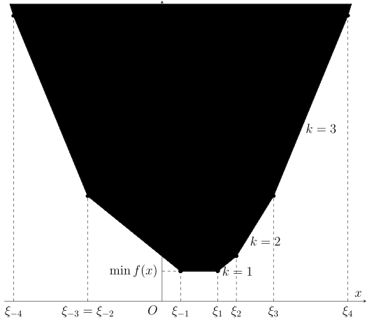
Example: minimum-cost increasing sequence
[BalticOI 2004] Sequence
Given a sequence \(\{a_i\}\) of length \(n\), find a strictly increasing sequence \(\{b_i\}\) that minimizes \(\sum_i|a_i-b_i|\). Output the minimum and any optimal \(\{b_i\}\).
Solution
First, \(\{b_i\}\) is strictly increasing if and only if \(\{b'_i\}=\{b_i-i\}\) is weakly increasing. So we find the weakly increasing sequence \(\{b'_i\}=\{b_i-i\}\) with the smallest total difference from \(\{a'_i\}=\{a_i-i\}\) and then recover \(\{b_i\}\) from it.
Start with the naive DP solution. Suppose the first \(i\) numbers of \(\{b'_i\}\) have been chosen and the \(i\)-th is at most \(x\). Let \(f_i(x)\) be the minimum total difference between the chosen numbers and the first \(i\) numbers of \(\{a'_i\}\):
The recurrence is
The initial state is \(f_0(x)\equiv 0\), and the answer is \(\min_xf_n(x)\). In terms of the transformations of convex functions described above, going from \(f_{i-1}(x)\) to \(f_i(x)\) takes two steps:
- First add \(|a'_i-x|\). This adds \(-1\) to the slope of every piece in the interval \((-\infty,a'_i]\) and adds \(1\) to the slope of every piece in the interval \([a'_i,+\infty)\).
- Then take a minimum of the result, turning \(g(x)=f_{i-1}(x)+|a'_i-x|\) into \(f_i(x)=\min_{y\le x}g(y)\). By the analysis above, this is the infimal convolution of \(g(x)\) and \(0_{[0,+\infty)}\). The latter has a single piece, of slope \(0\) and extending infinitely far to the right, so inserting it among the pieces of \(g(x)\) amounts to deleting every piece of positive slope.
With the operations spelled out, we could already maintain all the pieces in a balanced tree, but the code would be complicated. In this problem the slope changes by at most \(1\) at a time, so every slope is at most \(n\) in absolute value. It is easier to maintain the breakpoints than the pieces themselves.
Let the breakpoints of \(f_{i-1}(x)\) be \(\xi_{-k}\le\cdots\le\xi_{-1}\le\xi_{1}\le\cdots\le\xi_{\ell}\). The two steps above become:
- add \(a'_i\) once as a breakpoint of the negative-slope pieces and once as a breakpoint of the positive-slope pieces;
- pop all the breakpoints \(\xi_1,\cdots,\xi_{\ell}\) of the positive-slope pieces.
In an implementation, no breakpoints of positive-slope pieces are left after each round, so the breakpoints have the form \(\xi_{-k}\le\cdots\le\xi_{-1}\), and the operations always happen where the negative and positive slopes meet. A single max-heap that stores all the breakpoints is therefore enough. The two steps become:
- insert \(a'_i\) twice;
- pop the top of the heap.
We also have to keep track of the minimum of the current function after each round. Once a round is over there are no positive-slope pieces, so the minimum is the value of the function at the top of the max-heap. Suppose that before a round the top of the heap is \(\xi_{-1}\) and the minimum is \(f_{i-1}(\xi_{-1})\). The top that gets popped is the smallest breakpoint of the positive-slope pieces, and the minimum of the function equals its value there. So we simply evaluate the function at the top of the heap just before the pop:
The first terms are equal because \(f_{i-1}(x)\) has no positive-slope pieces. So each round only has to add \(\max\{0,\xi_{-1}-a'_i\}\) to the minimum.
The problem also asks for an optimal solution. When the last round is over, the optimum is the top of the heap, which determines \(b'_n\) directly. Now suppose the \(i\)-th optimal value \(b'_i\) is known and we want the best \(x\) for \(f_{i-1}(x)\) subject to \(x\le b'_i\). Since \(f_{i-1}(x)\) is convex, a solution is better the closer it is to the global minimum point. So it suffices to record the global minimum point of \(f_{i-1}(x)\) and take the smaller of it and \(b'_i\): this is the optimal \(b'_{i-1}\).
This runs in \(O(n\log n)\).
1 2 3 4 5 6 7 8 9 10 11 12 13 14 15 16 17 18 19 20 21 22 23 24 25 | |
Template problems:
- Codeforces 713 C. Sonya and Problem Without a Legend
- Luogu P2893 [USACO08FEB] Making the Grade G
- Luogu P4331 [BalticOI 2004] Sequence
- Luogu P4597 Sequence
- AtCoder 2nd Dwango Challenge Qualifier E - Fireworks
Example: constrained transitions
[NOISG 2018 Finals] Safety
Given a sequence \(\{a_i\}\) of length \(n\), find a sequence \(\{b_i\}\) that satisfies \(|b_i-b_{i-1}|\le h\) for all \(1<i\le n\) and minimizes \(\sum_i|a_i-b_i|\). Output the minimum.
Solution
This is much like the previous problem; only the constraint on the sequence \(\{b_i\}\) has changed. As before, let \(f_i(x)\) be the minimum total difference over the first \(i\) numbers when the \(i\)-th number is \(x\):
This gives the recurrence
The initial condition is \(f_0(x)\equiv 0\), and the answer is again \(\min_xf_n(x)\).
As operations on convex functions, the transition splits into two steps:
- first take a minimum of \(f_{i-1}(x)\), turning it into \(\min_{|y-x|\le h} f_{i-1}(y)\); this is the infimal convolution of \(f_{i-1}(x)\) and \(0_{[-h,h]}(x)\);
- then add \(|a_i-x|\) to the result.
Again the slope changes by only one at a time, so we maintain breakpoints. The two steps then read:
- shift all negative-slope pieces left by \(h\) and all positive-slope pieces right by \(h\);
- insert \(a_i\) twice.
In this problem it is convenient to maintain the negative-slope and the positive-slope pieces separately. The operations all take place near the piece of slope zero, so we use the two-heap technique: a max-heap holds the breakpoints of the negative-slope pieces and a min-heap those of the positive-slope pieces. A lazy tag shifts all the breakpoints of a heap at once. The second step inserts one \(a_i\) into each heap, and afterwards the top of the max-heap may exceed the top of the min-heap. In that case, swap the two tops until the order is restored.
Finally, the minimum has to be updated along the way. The shift in the first step does not change the minimum, so only the swaps of the tops matter. Suppose \(\xi_{-1}>\xi_1\). Swapping the tops \(\xi_{-1}\) and \(\xi_1\) changes the function from
to
The shape of the function stays the same; it only moves down by \(|\xi_{-1}-\xi_1|\). So to keep the function unchanged across the swap, add \(|\xi_{-1}-\xi_1|\) to the minimum.
The algorithm still runs in \(O(n\log n)\), because the tops are swapped at most once after each insertion.
1 2 3 4 5 6 7 8 9 10 11 12 13 14 15 16 17 18 19 20 21 22 23 24 25 26 27 28 29 30 31 32 33 34 35 | |
Template problems:
- Luogu P4272 [CTSC2009] Sequence Transformation
- Luogu P11598 [NOISG 2018 Finals] Safety
- AtCoder Beginner Contest 217 H - Snuketoon
- AtCoder Regular Contest 070 E - NarrowRectangles
- AtCoder Regular Contest 123 D - Inc, Dec - Decomposition
Maintaining slopes
In other problems it is easier to maintain the slopes. Such problems can usually also be solved with greedy with undo or by simulating a minimum-cost flow. In a minimum-cost flow model the minimum cost is typically a convex function of the flow, and this is what makes the slope trick applicable.
Example: stock trading
Codeforces 865 D. Buy Low Sell High
You are given the stock prices \(\{p_i\}\) (all positive) for \(n\) days. You start with \(0\) shares, and each day you may buy one share, sell one share or not trade. Find the maximum profit after \(n\) days.
Solution
Start with the naive DP solution. Let \(f_i(x)\) be the maximum profit at the end of day \(i\) when holding \(x\ge 0\) shares. Then
The initial state is \(f_0(0)=0\), with \(f_0(x)=-\infty\) for all \(x\neq 0\). The answer is \(f_n(0)\).
Going from \(f_{i-1}(x)\) to \(f_i(x)\) takes two steps:
-
Take the supremal convolution of \(f_{i-1}(x)\) and the piecewise linear function that corresponds to the function
\[ h_i(x) = \begin{cases}p_i,&x=-1,\\0,&x=0,\\-p_i,&x=1\end{cases} \]This piecewise linear function, \(\tilde h_i(x)\), is clearly concave.
-
The result has finite values on the interval \([-1,0)\), which contradicts the requirement \(x\ge 0\), so keep only the part of the function on \([0,+\infty)\).
In terms of linear pieces, these are the following two steps:
- insert a piece of length \(2\) and slope \(-p_i\);
- among the pieces of finite slope, delete a stretch of length \(1\) that has the largest slope.
The length of a piece is always a natural number, so we may as well maintain pieces of length one and record only the slope of each. The only operations needed are insertion and access to the maximum, so a max-heap is enough. There are two steps:
- insert \(-p_i\) twice;
- pop the top of the heap.
We also need to maintain the value of \(f_i(0)\). The function produced by the first step has the value \(f_{i-1}(0)+p_i\) at \(x=-1\), so its value at \(x=0\) is this value plus the top of the heap that is about to be popped, which is the slope of the function on the interval \([-1,0]\). Truncation does not change the value at \(x=0\), so this is \(f_i(0)\).
Comparing this implementation with the code for minimum-cost increasing sequence above shows that the algorithm is equivalent to finding the minimum cost of turning the stock prices into a weakly decreasing sequence.
This runs in \(O(n\log n)\).
1 2 3 4 5 6 7 8 9 10 11 12 13 14 15 16 17 18 19 20 | |
Template problems:
Example: moving earth
[USACO16OPEN] Landscaping P
You are given sequences \(\{a_i\}\) and \(\{b_i\}\) of length \(n\): the amount of dirt that garden \(i\) already has and the amount it needs (exactly, no more and no less). Buying one unit of dirt and putting it into any garden costs \(X\), carting one unit of dirt away from any garden costs \(Y\), and moving one unit of dirt from garden \(i\) to garden \(j\) costs \(Z|i-j|\). Find the minimum cost of meeting the needs of all gardens. (\(a_i,b_i\le 10\))
Solution
Start with the naive DP solution. Let \(f_i(x)\) be the minimum cost of meeting the needs of the first \(i\) gardens with a net surplus of \(x\) units of dirt to be moved on to the later gardens. If \(x<0\), there is a net deficit of \(|x|\) units of dirt that has to be brought in from the later gardens. The recurrence is
Here \(h(\delta)\) is the cost when the current garden makes a net purchase of \(\delta\) units of dirt:
It is clearly convex. The recurrence reads as follows:
- when the first \(i-1\) gardens have a net surplus of \(y\) units of dirt, the minimum cost is \(f_{i-1}(y)\);
- moving the net surplus (or deficit) between gardens \(i\) and \(i-1\) costs \(|y|Z\);
- the cheapest way of buying and removing dirt so that garden \(i\) goes from \(a_i\) to \(b_i\) units and the net surplus goes from \(y\) to \(x\) costs \(h((x-y)+(b_i-a_i))\).
The initial state is \(f_0(0)=0\), with \(f_0(x)=+\infty\) for all \(x\neq 0\). The answer is \(f_n(0)\).
Transforming the function \(f_{i-1}(x)\) into \(f_i(x)\) takes three steps:
- first add \(|x|Z\), which gives \(f_{i-1}(x)+|x|Z\);
- then take the infimal convolution with \(h(x)\), which gives \(\min_{y\in\mathbf R}f_{i-1}(y)+|y|Z+h(x-y)\);
- finally shift the function left by \((b_i-a_i)\) units.
As operations on the linear pieces, these are again three steps:
- add \(-Z\) to every piece left of the origin and \(Z\) to every piece right of the origin;
- replace every slope smaller than \(-Y\) by \(-Y\) and every slope larger than \(X\) by \(X\);
- shift all the pieces left by \((b_i-a_i)\) units.
In the original problem \(a_i\) and \(b_i\) are small, so it suffices to maintain pieces of length \(1\). There are infinitely many of them, but their slopes are bounded above by \(X\) and below by \(-Y\), and only a few slopes lie strictly between the two bounds. No insertions are involved, so two stacks can hold the pieces on the two sides of the origin, with the range additions and the range chmin/chmax all done by lazy tags. The three steps above become:
- put a lazy tag on each of the two stacks: add \(-Z\) on the left and \(Z\) on the right;
- whenever an element is popped from a stack, take its maximum with \(-Y\) and its minimum with \(X\). If the left stack is empty, pop \(-Y\). If the right stack is empty, pop \(X\);
- pop the top \((b_i-a_i)\) elements of the left stack and push them onto the right stack; when \(b_i-a_i<0\), do the reverse.
Update the answer as elements move between the stack tops: subtract the current slope when moving left and add the current slope when moving right.
The algorithm runs in \(O(n\max\{a_i,b_i\})\).
1 2 3 4 5 6 7 8 9 10 11 12 13 14 15 16 17 18 19 20 21 22 23 24 25 26 27 28 29 30 31 32 33 34 35 36 37 | |
Template problems:
- Luogu P2748 [USACO16OPEN] Landscaping P
- Kyoto University PC 2016 H - WAAAAAAAAAAAAALL
- JAG Practice Contest 2017 J - Farm Village
Practice problems
To close, here are some problems from various competitive programming contests that can be solved with the slope trick.
- Luogu P3642 [APIO2016] Fireworks Show
- Luogu P9962 [THUPC 2024 Preliminary Round] A Tree
- AtCoder Beginner Contest 383 G - Bar Cover
- Codeforces 280 D. k-Maximum Subsequence Sum
- Codeforces 280 E. Sequence Transformation
- Codeforces 802 O. April Fools' Problem (hard)
- Codeforces 1209 H. Moving Walkways
- Codeforces 1229 F. Mateusz and Escape Room
- Codeforces 1534 G. A New Beginning
- Codeforces 1787 H. Codeforces Scoreboard
- 2019 Summer Petrozavodsk Camp H. Honorable Mention
- 2018 ACM-ICPC World Finals C. Conquer The World
- 300iq Contest 3 F. Farm of Monsters
References and notes
- [Tutorial] Slope Trick - zscoder
- Slope trick explained - Kuroni
- Slope Trick - USACO Guide
- [Tutorial] Intuition on Slope Trick - maomao90
This page is an unofficial English translation of the original OI Wiki page (revision a9a6a11e), machine-translated by Claude Fable 5.2 on 2026-11-16. It has been modified from the original by translation and may contain errors. It is not endorsed by OI Wiki.
Found a translation problem? Report it on GitHub.
Authors of the original page: c-forrest, Tiphereth-A (full contribution history)
All content on this page is provided under the terms of CC BY-SA 4.0 and SATA; additional terms may apply.