Linear Basis
Recall the basis vectors of high-school solid geometry: in three-dimensional Euclidean space we can pick basis vectors \(\boldsymbol{i}\), \(\boldsymbol{j}\), \(\boldsymbol{k}\), and every vector of the space can then be expressed in terms of them. In other words, a finite number of basis vectors describes an infinite three-dimensional space, which shows how important basis vectors are.
Three-dimensional Euclidean space is a special case of a vector space; the linear basis generalizes its basis vectors to arbitrary vector spaces.
In OI, applications of the linear basis usually involve only two kinds of vector space: the \(n\)-dimensional real vector space \(\mathbf{R}^n\) and the \(n\)-dimensional vector space \(\mathbf{Z}_2^n\) over the Boolean domain. The Applications section covers them in detail. If you are not familiar with linear algebra, start reading there.
Below we introduce the linear basis for a general vector space and give its common properties.
Prerequisite reading: vector spaces.
A linear basis is a basis of a vector space, and an important tool for studying vector spaces.
Definition
A maximal linearly independent set of a vector space \(V\) is called a Hamel basis or linear basis of \(V\), or simply a basis.
By convention, the basis of the vector space \(\{\theta\}\) is the empty set.
One can show that every vector space has a linear basis1. The dimension of a vector space \(V\), written \(\dim V\), is the number of elements (or the cardinality) of a linear basis.
Properties
-
Let \(V\) be a finite-dimensional vector space of dimension \(n\). Then:
-
Any \(n+1\) vectors of \(V\) are linearly dependent.
-
Any \(n\) linearly independent vectors of \(V\) form a basis of \(V\).
-
If every vector of \(V\) is a linear combination of the vectors \(a_1,a_2,\dots,a_n\), then these form a basis of \(V\).
Proof
Take any basis \(b_1,b_2,\dots,b_n\) of \(V\). By assumption, \(b_1,b_2,\dots,b_n\) are linear combinations of \(a_1,a_2,\dots,a_n\), so
\[ n=\operatorname{rank}\{b_1,b_2,\dots,b_n\}\leq\operatorname{rank}\{a_1,a_2,\dots,a_n\}\leq n \]Hence \(\operatorname{rank}\{a_1,a_2,\dots,a_n\}=n\).
-
Any linearly independent vectors \(a_1,a_2,\dots,a_m\) of \(V\) can be extended to a basis of \(V\) by adding some vectors.
-
-
(Dimension formula for subspaces) Let \(V_1,V_2\) be finite-dimensional vector spaces over \(\Bbb{P}\) such that \(V_1+V_2\) and \(V_1\cap V_2\) are also finite-dimensional. Then \(\dim V_1+\dim V_2=\dim(V_1+V_2)+\dim(V_1\cap V_2)\).
Proof
Let \(\dim V_1=n_1\), \(\dim V_2=n_2\) and \(\dim(V_1\cap V_2)=m\).
Take a basis \(a_1,a_2,\dots,a_m\) of \(V_1\cap V_2\) and extend it to a basis of \(V_1\) and to a basis of \(V_2\): \(a_1,a_2,\dots,a_m,b_1,b_2,\dots,b_{n_1-m}\) and \(a_1,a_2,\dots,a_m,c_1,c_2,\dots,c_{n_2-m}\).
It remains to show that the vectors \(a_1,a_2,\dots,a_m,b_1,b_2,\dots,b_{n_1-m},c_1,c_2,\dots,c_{n_2-m}\) are linearly independent.
Suppose \(\sum_{i=1}^m r_ia_i+\sum_{i=1}^{n_1-m} s_ib_i+\sum_{i=1}^{n_2-m} t_ic_i=\theta\).
Then \(\sum_{i=1}^{n_2-m} t_ic_i=-\sum_{i=1}^m r_ia_i-\sum_{i=1}^{n_1-m} s_ib_i\).
The left-hand side lies in \(V_2\) and the right-hand side in \(V_1\), so both lie in \(V_1\cap V_2\), and therefore \(\sum_{i=1}^{n_2-m} t_ic_i=\sum_{i=1}^m k_ia_i\).
Hence \(t_1=t_2=\dots=t_{n_2-m}=k_1=k_2=\dots=k_m=0\), and so \(r_1=r_2=\dots=r_m=s_1=s_2=\dots=s_{n_1-m}=t_1=t_2=\dots=t_{n_2-m}=0\).
-
Let \(V_1,V_2\) be finite-dimensional vector spaces over \(\Bbb{P}\) such that \(V_1+V_2\) and \(V_1\cap V_2\) are also finite-dimensional. Then the following are equivalent:
-
\(V_1+V_2=V_1\oplus V_2\).
-
\(\dim V_1+\dim V_2=\dim(V_1+V_2)\).
-
If \(a_1,a_2,\dots,a_n\) is a basis of \(V_1\) and \(b_1,b_2,\dots,b_m\) is a basis of \(V_2\), then \(a_1,a_2,\dots,a_n,b_1,b_2,\dots,b_m\) is a basis of \(V_1+V_2\).
Note
Items 1 and 3 extend to infinite-dimensional vector spaces.
-
Example
Consider bases of \(\Bbb{R}^2\).
-
In the figure
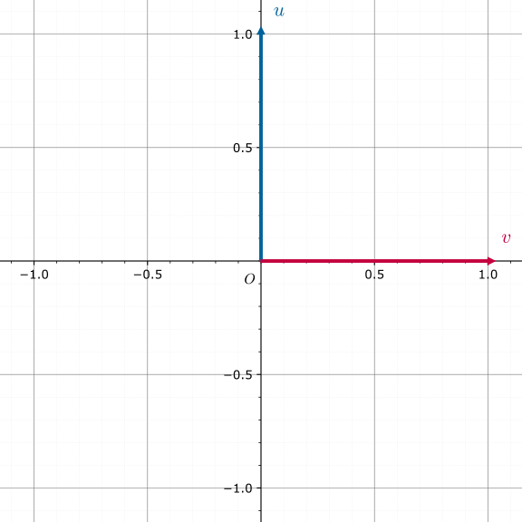
\(u,v\) form a basis.
-
In the figure
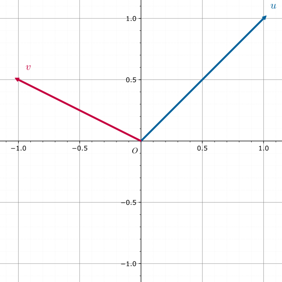
\(u,v\) form a basis.
-
In the figure
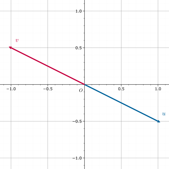
\(u,v\) do not form a basis, because \(u=-v\).
-
In the figure
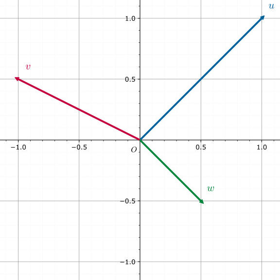
\(u,v,w\) do not form a basis, because \(u+4v+6w=\theta\).
Orthogonal and orthonormal bases
A basis \(B\) of a vector space \(V\) is an orthogonal basis if \(\forall b,b'\in B,~(b,b')\ne 0\iff b=b'\), that is, if its vectors are pairwise orthogonal.
An orthogonal basis \(B\) of a vector space \(V\) is an orthonormal basis if it also satisfies \(\forall b\in B,~|b|=\sqrt{(b,b)}=1\).
Any basis of a finite-dimensional vector space \(V\) can be turned into an orthogonal basis by Gram–Schmidt orthogonalization.
Applications
By the above, a linear basis lets us:
- find the rank of a given set of vectors;
- find a maximal linearly independent subset of a given set of vectors (or a basis of the vector space it spans);
- insert vectors into a given set of vectors and find a maximal linearly independent subset of the resulting set (or a basis of the vector space it spans);
- given a maximal linearly independent subset (or basis) found in this way, decide whether a vector is a linear combination of it;
- given a maximal linearly independent subset (or basis) found in this way, find special elements of the vector space it spans, such as the largest or the smallest.
In OI, a linear basis of the \(n\)-dimensional real vector space \(\mathbf{R}^n\) is usually called a real basis, and a linear basis of the \(n\)-dimensional vector space \(\mathbf{Z}_2^n\) over the Boolean domain an XOR basis.
Tip
Addition in \(\mathbf{Z}_2\) is XOR and multiplication is AND; one can show that \(\mathbf{Z}_2\) is a field.
One can also show that the algebraic structure \((\mathbf{Z}_2^n,+,\cdot,\mathbf{Z}_2)\) is a vector space, where:
That is, addition is XOR and scalar multiplication is AND.
Take the XOR basis as an example. From a given set of Boolean sequences \(X=\{x_1,\dots,x_m\}\) we can construct an XOR basis \(B=\{b_1,\dots,b_n\}\) with the following properties:
- no non-empty subset of \(B\) has XOR sum \(0\);
- every element \(x\) of \(X\) is the XOR sum of some elements of \(B\);
- any set \(B'\) with the two properties above has at least as many elements as \(B\).
An XOR basis lets us:
- decide whether a number is the XOR sum of a subset of a given set of numbers;
- find the number of ways to write a number as the XOR sum of a subset of a given set of numbers;
- find the maximum, minimum, \(k\)-th largest or \(k\)-th smallest XOR sum over the subsets of a given set of numbers;
- find the rank of a number among the subset XOR sums of a given set of numbers.
Construction
An XOR basis and a real basis do not differ in any essential way, so we work with the XOR basis from here on; the code for a real basis needs only a few simple changes.
Greedy method
Write each number \(p\) of the original set in binary and scan it from the high bits to the low bits. At each bit \(x\) that is \(1\): if \(a_x\) does not exist, set \(a_x \leftarrow p\) and stop scanning; if it exists, set \(p\leftarrow p~\text{xor}~a_x\).
To find the maximum \(\text{xor}\) of any number of elements of the original set, scan the linear basis from the high bits to the low bits: whenever taking the answer \(\text{xor}\) the current \(a_x\) makes it larger, XOR \(a_x\) into the answer.
Why does this work? Because the scan goes from high to low: reaching bit \(i\) means that we can make bit \(i\) of the answer \(1\), and nothing later gets a chance to change bit \(i\).
For the minimum \(\text{xor}\) of any number of elements of the original set: if some number was reduced to \(0\) during insertion, the minimum is \(0\); otherwise it is the smallest element of the linear basis.
To check whether a number can be obtained as an XOR, proceed as in insertion: if the number \(p\) being inserted ends up reduced to \(0\), it can.
Code (Luogu P3812 [Template] Linear Basis)
1 2 3 4 5 6 7 8 9 10 11 12 13 14 15 16 17 18 19 20 21 22 23 24 25 26 27 28 29 30 31 32 33 34 35 36 | |
Gaussian elimination
Gaussian elimination builds the linear basis from the point of view of a system of linear equations; its correctness is clear.
Code (Luogu P3812 [Template] Linear Basis)
1 2 3 4 5 6 7 8 9 10 11 12 13 14 15 16 17 18 19 20 21 22 23 24 25 26 27 28 29 30 31 32 33 34 35 36 37 38 39 | |
Properties
A linear basis built by the greedy method has the following properties:
- No non-empty subset of the basis has XOR sum \(0\).
- The numbers in the basis have pairwise distinct highest set bits.
A linear basis built by Gaussian elimination has the following property:
-
The matrix after Gaussian elimination is in reduced row echelon form.
This property implies both properties of a linear basis built by the greedy method.
If you do not see why this property holds, see Gaussian elimination.
Here is a sample:
1 2 | |
In binary:
1 2 3 4 5 | |
The linear basis produced by the greedy method:
1 2 3 4 5 6 7 8 9 10 | |
The linear basis produced by Gaussian elimination:
1 2 3 4 5 6 7 8 9 10 | |
This is a very useful property, and it makes many problems easier. For example: given some numbers, choose some of them so that their XOR is as large as possible. With a basis built by the greedy method you need a second greedy pass: if the current bit of ans is 0, XORing always improves the answer, and if the current bit is 1, it never does. With a basis built by Gaussian elimination you just XOR all elements of the basis together and output the result.
A basis obtained by Gaussian elimination also makes the other classic problems easier (whether a number can be obtained as an XOR, the \(k\)-th largest number that can be obtained as an XOR, and so on).
Time complexity
Let \(n\) be the length of a vector and \(m\) the number of vectors. The time complexity is \(O(nm)\); Gaussian elimination has a slightly larger constant factor.
For a real basis the time complexity is \(O(n^2m)\).
Merging linear bases
Linear bases are merged by brute force: insert the vectors of one basis into the other, one by one. A single merge takes \(O(n^2)\) time (XOR basis) or \(O(n^3)\) time (real basis).
Intersecting linear bases
Strictly speaking, intersecting two linear bases means finding a linear basis of the intersection of the two vector spaces they span. This section presents two algorithms. Both compute a single intersection in \(O(n^2)\) time (XOR basis) or \(O(n^3)\) time (real basis).
Naive algorithm
Let \(\alpha\) and \(\beta\) be the linear bases to intersect. The intersection algorithm is the brute-force merge with the following changes (described for an XOR basis):
- Try to insert each vector \(\beta_j\) of the linear basis \(\beta\) into \(\alpha\) by the greedy method, and initialize the intersection basis \(\gamma\) to the empty set.
- During an insertion, keep track of the contribution of the elements of \(\beta\) to the vector being inserted. Concretely, maintain a new vector \(b\), initially \(\beta_j\); whenever the vector being inserted is XORed with the basis vector at bit \(x\), XOR the contribution \(b\) with the contribution \(b_x\) recorded at bit \(x\) as well.
- If the insertion succeeds and puts a vector \(\beta_j'\) at bit \(x\) of the basis, set the \(b_x\) recorded at bit \(x\) to \(b\), the contribution of the elements of \(\beta\) to \(\beta_j'\).
- If the insertion fails, insert the contribution \(b\) of the elements of \(\beta\) recorded along the way into \(\gamma\).
The resulting linear basis \(\gamma\) is the intersection we want. The algorithm of course computes the union of the two bases as well.
Explanation of the algorithm
Let the merged basis be \(\{\alpha_1,\cdots,\alpha_m,\beta'_{j_1},\cdots,\beta'_{j_\ell}\}\), where \(\beta'_{j_k}\) is the vector finally obtained when \(\beta_{j_k}\) is inserted. Then \(\{\alpha_1,\cdots,\alpha_m,\beta_{j_1},\cdots,\beta_{j_\ell}\}\) is a merged basis too. Write \(\beta^+\) for the set \(\{\beta_{j_1},\cdots,\beta_{j_\ell}\}\), so that the merged basis is \(\alpha\cup\beta^+\). Every vector \(c\) of the sum space can then be written uniquely as
with \(a\in\operatorname{span}\alpha\) and \(b\in\operatorname{span}\beta^+\). The \(b\) of this decomposition is what the algorithm above tries to record as "the contribution of the elements of \(\beta\)". Strictly speaking, it is only the contribution of those vectors of \(\beta\) that end up being inserted successfully.
For a successful insertion, the \(b\) recorded at the end is the \(b\) term of this decomposition. Let \(\beta_j\in\beta^+\). Initially \(\beta_j=0\oplus\beta_j\), which is already the correct decomposition of \(\beta_j\) over the basis \(\alpha\cup\beta^+\). When \(\beta'_j=a\oplus b\) is updated to \(\beta'_j\oplus c_x\), we have \(\beta_j'\oplus c_x=(a\oplus a_x)\oplus(b\oplus b_x)\), so updating \(b\) to \(b\oplus b_x\) is enough to keep the decomposition correct. By induction, when \(\beta'_j\) is finally inserted into the merged basis, the recorded contribution \(b\) is the \(b\) term of the decomposition above.
For a failed insertion, the vector being inserted always ends up as \(0\), and the contribution \(b\) at that point is inserted into \(\gamma\). Repeating the argument above shows that \(\beta_j'=a\oplus b\) with \(a\in\operatorname{span}\alpha\) still holds throughout the insertion; only \(b\) no longer belongs to \(\operatorname{span}\beta^+\). The reason is that the initial decomposition \(\beta_j=0\oplus\beta_j\) now has \(\beta_j\notin\beta^+\). Apart from that, every term XORed into the contribution during an update belongs to \(\operatorname{span}\beta^+\). So in fact \(b\oplus\beta_j\in\operatorname{span}\beta^+\).
Why, then, does inserting the \(b\) of every failed insertion into \(\gamma\) give a linear basis of the intersection? First, a failed insertion of \(\beta_j\) always ends with \(0=a\oplus b\), where \(a\in\operatorname{span}\alpha\) and \(b\in\operatorname{span}(\beta^+\cup\{\beta_j\})\subseteq\operatorname{span}\beta\). Hence \(b=a\) lies in the intersection \(\operatorname{span}\alpha\cap\operatorname{span}\beta\). Conversely, let \(c\) be any element of the intersection. Since \(c\in\operatorname{span}\beta\), it is a linear combination (an XOR sum) of elements of \(\beta\):
where \(\lambda_j\in\{0,1\}\). For each \(\beta_j\notin\beta^+\), let \(b_j\) be the corresponding contribution inserted into \(\gamma\). Then
Both \(b_j\) and \(c\) lie in the intersection, so the left-hand side does too, and it can therefore be written as a linear combination of elements of \(\alpha\). On the right-hand side, every term has either \(\beta_j\in\beta^+\), or \(\beta_j\notin\beta^+\) and \(\beta_j\oplus b_j\in\beta^+\), so the right-hand side is in fact a linear combination of elements of \(\beta^+\). But \(\alpha\cup\beta^+\) is linearly independent, so all the coefficients are \(0\); that is, \(c=\bigoplus_{\beta_j\notin\beta^+}\lambda_jb_j\in\operatorname{span}\{b_1,\cdots,b_j\}\). This shows that the contributions \(b\) of the vectors that could not be inserted together span the intersection.
By this explanation, the real purpose of maintaining the contribution \(b\) is to maintain the decomposition \(a\oplus b\); and whenever a contribution is finally inserted into \(\gamma\), we have \(a=b\). So the result is correct whether we track the contribution of the elements of \(\alpha\) or of \(\beta\) (that is, whether we maintain \(a\) or \(b\)). To track the contribution of the elements of the linear basis \(\alpha\) instead, change only the initial values of the contributions: each vector \(\alpha_i\) of \(\alpha\) starts with contribution \(\alpha_i\), and an inserted \(\beta_j\) starts with contribution \(0\).
Code for the template problem:
Code (Library Checker Intersection of \(\mathbf F_2\) vector spaces)
1 2 3 4 5 6 7 8 9 10 11 12 13 14 15 16 17 18 19 20 21 22 23 24 25 26 27 28 29 30 31 32 33 34 35 36 37 38 39 40 41 42 43 44 45 46 47 48 49 50 51 52 53 54 55 56 57 58 59 60 61 62 63 64 65 66 67 68 69 70 71 72 73 74 75 76 77 78 79 80 81 82 83 84 85 86 87 88 89 | |
Zassenhaus algorithm
An equivalent alternative is the Zassenhaus algorithm, which likewise computes the union and the intersection of two linear bases at the same time. Its complexity is exactly the same as above.
The steps are:
- Initialize an empty linear basis \(\gamma\) of vectors of length \(2n\), each written as \((a,b)\) with \(a\) and \(b\) both of length \(n\).
- Insert each element \(\alpha_i\) of \(\alpha\) into \(\gamma\) as \((\alpha_i,\alpha_i)\).
- Insert each element \(\beta_j\) of \(\beta\) into \(\gamma\) as \((\beta_j,0)\).
- Consider the nonzero elements \((c_k,d_k)\) of the final linear basis \(\gamma\). The components \(c_k\) of the vectors with \(c_k\) nonzero form a linear basis of the union of \(\alpha\) and \(\beta\), and the components \(d_k\) of the vectors with \(c_k\) zero form a linear basis of the intersection of \(\alpha\) and \(\beta\).
The linear basis in the algorithm can be built by the greedy method or by Gaussian elimination, as long as the basis in \(\gamma\) forms a matrix in row echelon form.
Comparing the elimination steps of the Zassenhaus algorithm with the naive algorithm above shows that the Zassenhaus algorithm built on the greedy method is exactly the naive algorithm that tracks the contribution of the elements of \(\alpha\). If we instead insert all the \((\alpha_i,0)\) first and then all the \((\beta_j,\beta_j)\), the greedy Zassenhaus algorithm becomes the naive algorithm that tracks the contribution of the elements of \(\beta\). Since the elimination steps are equivalent, the Zassenhaus algorithm is correct as well.
There is also an independent and more general algebraic proof:
Proof of correctness
Let \(V\) be a vector space with subspaces \(U=\operatorname{span}\alpha\) and \(W=\operatorname{span}\beta\). In effect, the algorithm reduces to row echelon form the generators of the subspace
and thereby finds a basis \(\gamma\) of it. At the end of the algorithm, the elements \((c_k,d_k)\) of \(\gamma\) are split into two classes according to whether \(c_k\neq 0\), so consider the projection \(\pi:H\rightarrow V\) with \(\pi(a,b)=a\). Then \(\pi(H)=U+W\), and it is easy to check that
By the theorem on linear maps, \(\dim H = \dim\pi(H)+\dim\ker\pi = \dim(U+W)+\dim(U\cap W)\).
The first few columns of a matrix in row echelon form again form a matrix in row echelon form, so the number of rows with \(c_k\neq 0\) is exactly the row rank of \(\alpha\cup\beta\), that is, \(\dim(U+W)\); moreover, the \(c_k\) of these rows form a basis of \(U+W\). Exactly \(\dim(U\cap W)\) nonzero rows remain, and they all have \(c_k=0\). For the \(d_k\) of these rows, \((0,d_k)\in\ker\pi\) gives \(d_k\in U\cap W\); and the \((0,d_k)\), being rows of a matrix in row echelon form, are linearly independent, so these \(d_k\) are linearly independent too. Altogether, these \(d_k\) are a linearly independent set of size \(\dim(U\cap W)\) in the intersection \(U\cap W\), and hence a basis of it.
Code for the template problem:
Code (Library Checker Intersection of \(\mathbf F_2\) vector spaces)
1 2 3 4 5 6 7 8 9 10 11 12 13 14 15 16 17 18 19 20 21 22 23 24 25 26 27 28 29 30 31 32 33 34 35 36 37 38 39 40 41 42 43 44 45 46 47 48 49 50 51 52 53 54 55 56 57 58 59 60 61 62 63 64 | |
Note that only the vectors whose first \(n\) bits are all zero need to be output.
Extension: prefix linear basis
This section treats only the XOR basis, and assumes that a single vector fits in \(O(1)\) space and that a single operation always takes \(O(1)\) time.
When the maximum XOR of a range has to be queried many times, a common approach combines a cat tree with linear bases and takes \(O(nm\log m+n^2q)\) time, where \(n\) is the length of a vector, \(m\) the length of the sequence and \(q\) the number of queries. Another approach uses a prefix linear basis (also called a timestamped linear basis), which lowers the complexity to \(O(n(m+q))\).
A prefix linear basis maintains, for every prefix of the sequence, the linear bases of all suffixes of that prefix, so it can answer a query for the linear basis of any range. The linear bases of the suffixes \([j,i]\) of a prefix \([1,i]\) are nested: the basis of \([j,i]\) always contains the basis of \([j+1,i]\). So at most \(n\) of these suffix bases are pairwise distinct, and all of them, from \([i,i]\) to \([1,i]\), can be obtained by adding new vectors to the empty set one at a time. Thanks to this monotonicity, it is enough to label each added vector \(v\) with the largest index \(t\) at which it appears; the linear bases of all the suffixes then fit in \(O(n)\) space. To get the linear basis of a range \([j,i]\), keep only the vectors with label \(t\ge j\) in the prefix linear basis at \(i\).
Call the label \(t\) of a vector \(v\) its timestamp. A vector \(v\) of the linear basis can always be written as the XOR sum of some elements of the original sequence, say \(v_{i_1}\oplus v_{i_2}\oplus\cdots\oplus v_{i_k}\). Over all such representations, the largest possible value of the smallest index is \(t\), that is,
This expression merely restates the previous paragraph in formal language. What it suggests is that, to maintain the timestamp of every vector \(v\) of the linear basis, we only have to greedily replace old vectors by vectors that are as new as possible.
Starting from the greedy method described above, the construction of a prefix linear basis makes the following changes:
- Store a timestamp \(t_x\) with each vector \(a_x\) kept in the linear basis, initially \(0\).
- To add the \(i\)-th vector \(v\) of the sequence, still scan from the high bits to the low bits, but also keep track of the current time \(i\).
- If bit \(x\) of \(v\) is one, compare the timestamp \(t_x\) of the vector \(a_x\) already in the linear basis with the current time \(i\):
- If \(i>t_x\), the vector being added is newer: set \(a_x\) to \(v\) and its timestamp to \(i\), then continue the process with \(a_x\oplus v\), the XOR of the old \(a_x\) and \(v\), at the previously recorded time \(t_x\).
- If \(i<t_x\), the vector being added is older: leave \(a_x\) and \(t_x\) unchanged, XOR \(v\) with \(a_x\) and continue.
In other words, if the current bit can be represented by a newer vector, use the newer vector; otherwise keep the old one. When updating the vector at bit \(x\), do not store the XOR \(a_x\oplus v\) there, because its timestamp is \(\min\{t(a_x),t(v)\}=t(a_x)\), which is smaller than the timestamp \(t(v)\) of the vector \(v\) being added. For the same reason, the upward updates of Gaussian elimination may break the timestamp property, so it can no longer be used to build a prefix linear basis.
Code for the template problem:
Code (Codeforces 1100F Ivan and Burgers)
1 2 3 4 5 6 7 8 9 10 11 12 13 14 15 16 17 18 19 20 21 22 23 24 25 26 27 28 29 30 31 32 33 34 35 36 37 38 39 40 41 42 43 44 45 46 47 48 49 50 51 52 53 54 55 56 57 58 59 60 61 62 | |
If queries must be answered online, you can instead store the prefix linear basis at every prefix, using \(O(mn)\) space, and then query; this can be viewed as a kind of "persistent" linear basis. If you need the properties of a linear basis obtained by Gaussian elimination, handle that separately at query time.
Practice problems
- Luogu P3812 [Template] Linear Basis
- AcWing 3164. Linear Basis
- SGU 275 to xor or not xor
- HDU 3949 XOR
- HDU 6579 Operation
- Luogu P4151 [WC2011] Maximum XOR Sum Path
- Library Checker - Intersection of \(\mathbf F_2\) vector spaces
- AtCoder Grand Contest 045 A - Xor Battle
- Codeforces 1100F Ivan and Burgers
- Luogu P3292 [SCOI2016] Lucky Numbers
References and notes
- Weisheng Qiu. Advanced Algebra (Volume 2) (in Chinese). Tsinghua University Press.
- Basis (linear algebra) - Wikipedia
- Vector Basis -- from Wolfram MathWorld
- Zassenhaus algorithm - Wikipedia
This page is an unofficial English translation of the original OI Wiki page (revision 9bb3a8e6), machine-translated by Claude Fable 5.2 on 2026-11-16. It has been modified from the original by translation and may contain errors. It is not endorsed by OI Wiki.
Found a translation problem? Report it on GitHub.
Authors of the original page: cesonic, Enter-tainer, Great-designer, Ir1d, ksyx, lychees, MegaOwIer, RUIN-RISE, wjy-yy, rsdbkhusky, ouuan, Menci, Tiphereth-A, 24OI-bot, iamtwz, Xeonacid, Persdre, shuzhouliu, CoelacanthusHex, aofall, Marcythm, c-forrest, yusancky, hensier, Plastic-time (full contribution history)
All content on this page is provided under the terms of CC BY-SA 4.0 and SATA; additional terms may apply.