Introduction to Complexity
Time complexity and space complexity are important measures of an algorithm's efficiency.
Number of basic operations
The same algorithm runs at different speeds on different computers. Its actual speed is hard to work out in theory and tedious to measure. So we usually consider not the actual running time of an algorithm but the number of basic operations it has to perform.
On an ordinary computer, the four arithmetic operations, accessing a variable (of a primitive type, here and below) and assigning to a variable all count as basic operations.
A count or an estimate of the basic operations serves as a measure of an algorithm's running time.
Time complexity
Definition
You cannot judge how fast an algorithm is without taking the input size into account. The input size usually means something like the number of values in the input, or the numbers of vertices and edges of a graph given in the input. In general, the larger the input, the longer the algorithm takes. In competitive programming, what matters most about an algorithm's efficiency is not its running time at one particular input size but how its running time grows with the input size. This is its time complexity.
Introduction
There are two main reasons to look at how the running time changes with the input size:
- A modern computer performs hundreds of millions of basic operations per second or more, so the inputs we deal with are usually large. Suppose algorithm A takes \(100n\) time on an input of size \(n\) and algorithm B takes \(n^2\). For inputs smaller than \(100\), B is faster. But in one second A can handle inputs with sizes in the millions, while B can only handle sizes in the tens of thousands. When the algorithm is allowed to run for longer, the effect of the time complexity on the input size it can handle becomes even more pronounced, and far outweighs the effect of the running time at any one input size.
- We measure running time by the number of basic operations, but different basic operations take different amounts of time: addition and subtraction, for example, are much faster than division. Time complexity ignores the differences between basic operations, as well as the difference between one basic operation and ten, and so removes the effect of their unequal costs.
Of course, an algorithm's running time is not determined by the input size alone: it also depends on the contents of the input. So time complexity comes in several kinds, for example:
- Worst-case time complexity: the time complexity given by the slowest input of each size. In competitive programming the input can be anything within the given constraints, and the algorithm must pass every input within them, so we usually consider the worst-case time complexity.
- Average-case (expected) time complexity: the complexity of the running time averaged over all possible inputs of each size (that is, of the expected running time under a given probability distribution over the inputs; the uniform average is a common special case).
"How the running time grows with the input size" is a vague notion. To express time complexity formally we need asymptotic notation, introduced below.
Definition of asymptotic notation
Asymptotic notation is the standard way to describe the order of growth of a function. Put simply, it ignores the slower-growing parts of a function and the coefficients of its terms (in complexity analysis these coefficients are usually called "constant factors"), and keeps the important part that shows how the function grows.
A simple mnemonic: the non-strict relations (which include equality) use capital letters, and the strict ones (which exclude it) use lowercase letters; equality is \(\Theta\), less-than is \(O\), and greater-than is \(\Omega\). Big \(O\) and little \(o\) were originally the Greek letter omicron, but since it has the same shape, they can just as well be read as the Latin letters \(O\) and \(o\).
In English, the roots "-micro-" and "-mega-" commonly denote 10 to the minus sixth power (one millionth) and 10 to the sixth power (one million), and they also mean "small" and "large". Small and large are also what the Greek letters omicron and omega usually stand for.
Big Θ notation
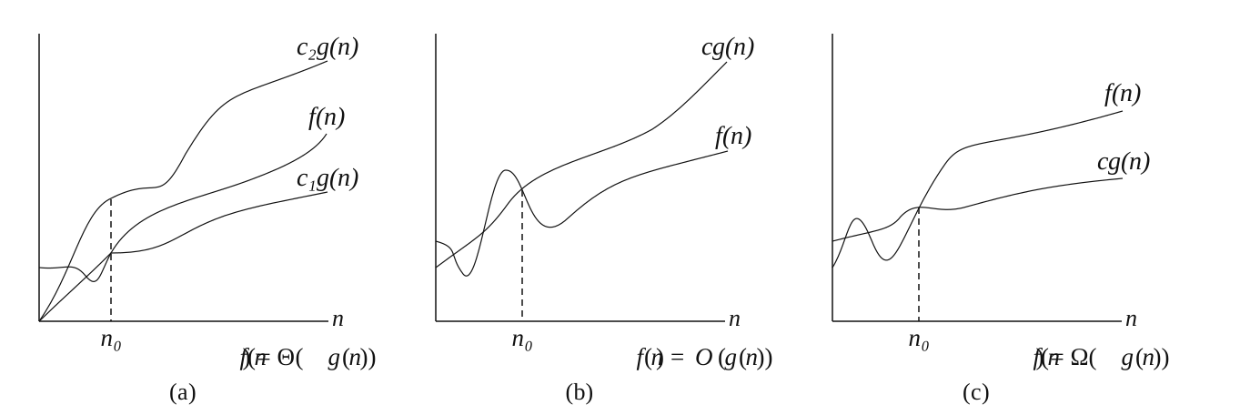
For functions \(f(n)\) and \(g(n)\), we have \(f(n)=\Theta(g(n))\) if and only if \(\exists c_1,c_2,n_0>0\) such that \(\forall n \ge n_0, 0\le c_1\cdot g(n)\le f(n) \le c_2\cdot g(n)\).
In other words, if \(f(n)=\Theta(g(n))\), we can find two positive numbers \(c_1, c_2\) such that \(f(n)\) is sandwiched between \(c_1\cdot g(n)\) and \(c_2\cdot g(n)\).
For example, \(3n^2+5n-3=\Theta(n^2)\), where \(c_1, c_2, n_0\) can be \(2, 4, 100\) respectively. Likewise \(n\sqrt {n} + n{\log^5 n} + m{\log m} +nm=\Theta(n\sqrt {n} + m{\log m} + nm)\): because \(\log^5 n=o(\sqrt n)\), there is a sufficiently large \(n_0\) beyond which the omitted term is at most \(n\sqrt n\).
Big O notation
\(\Theta\) notation bounds a function from above and from below at once. If we know only an asymptotic upper bound of a function and not an asymptotic lower bound, we can use \(O\) notation. We have \(f(n)=O(g(n))\) if and only if \(\exists c,n_0>0\) such that \(\forall n \ge n_0,0\le f(n)\le c\cdot g(n)\).
Time complexity is usually studied with \(O\) notation, because we normally care about an upper bound on a program's running time, not a lower bound.
Note that "upper bound" and "lower bound" here refer to how a function grows, not to the algorithm. The upper bound on an algorithm's running time corresponds to its "worst-case time complexity", not to big \(O\) notation. So it is perfectly fine to state a worst-case time complexity with \(\Theta\) notation, and \(\Theta\) is arguably more precise than \(O\). There are two main reasons for using \(O\) notation anyway: first, sometimes we can prove only an upper bound on the time complexity and not a lower bound (this tends to happen with more complicated algorithms and complexity analyses); second, \(O\) is easier to type on a computer.
Big Ω notation
Similarly, we use \(\Omega\) notation to describe an asymptotic lower bound of a function. We have \(f(n)=\Omega(g(n))\) if and only if \(\exists c,n_0>0\) such that \(\forall n \ge n_0,0\le c\cdot g(n)\le f(n)\).
Little o notation
If \(O\) notation corresponds to the less-than-or-equal sign, then \(o\) notation corresponds to the less-than sign.
Little \(o\) notation is used heavily in mathematical analysis. The Taylor expansion of a function at a point has a Peano remainder, which uses little \(o\) to express "strictly smaller"; this is the basis of asymptotic analysis with equivalent infinitesimals.
We have \(f(n)=o(g(n))\) if and only if for every positive number \(c\), \(\exists n_0\) such that \(\forall n \ge n_0,0\le f(n)< c\cdot g(n)\).
Little ω notation
If \(\Omega\) notation corresponds to the greater-than-or-equal sign, then \(\omega\) notation corresponds to the greater-than sign.
We have \(f(n)=\omega(g(n))\) if and only if for every positive number \(c\), \(\exists n_0\) such that \(\forall n \ge n_0,0\le c\cdot g(n)< f(n)\).
Common properties
- \(f(n) = \Theta(g(n))\iff f(n)=O(g(n))\land f(n)=\Omega(g(n))\).
- \(f_1(n) + f_2(n) = O(\max(f_1(n), f_2(n)))\).
- \(f_1(n) \times f_2(n) = O(f_1(n) \times f_2(n))\).
- \(\forall a>1, \log_a{n} = O(\log_2 n)\). By the change-of-base formula, logarithms to any fixed real base \(a>1\) all grow at the same rate, so the base of a logarithm is usually omitted in asymptotic time complexities.
Simple examples of computing time complexity
for loops
1 2 3 4 5 6 7 8 9 | |
1 2 3 4 5 6 | |
1 2 3 4 5 6 7 8 9 10 | |
If we take the values of the inputs \(n\) and \(m\) as the input size, the code above runs in \(\Theta(n^2m)\).
DFS
A DFS on a connected graph with \(n\) vertices and \(m\) edges, stored as adjacency lists, takes \(\Theta(n+m)\) time, because every vertex and every edge is visited only a constant number of times.
Which quantities are constants
When we perform some number of operations, how do we tell whether that number affects the time complexity? For example:
1 2 3 4 | |
1 2 3 | |
1 2 3 4 | |
If \(N\) is not regarded as part of the input size, this code runs in \(O(1)\).
When you compute a time complexity, it matters a great deal which variables count as the input size. Every quantity that does not depend on the input size is a constant and can be treated as \(1\) in the calculation.
Note that theoretical discussions of time complexity rest on the basic assumption that "the algorithm can solve problems of any size" (in practice, of course, time and memory are limited, so problems that are too large cannot be solved). So being able to solve problems of bounded size in constant time (for example, by precomputing the answer for every possible input within the constraints) does not make an algorithm's time complexity \(O(1)\).
Master theorem
The master theorem quickly gives the complexity of a recursive algorithm. Let \(a\ge1\) and \(b>1\) be constants, let \(f\) be nonnegative, and let \(T(1)=\Theta(1)\). To simplify the discussion, we also assume below that \(n=b^L\), where \(L\) is a nonnegative integer. The recurrence is
Then
Note that the second case also requires the regularity condition: there is a constant \(0<c<1\) such that \(a f(n/b) \leq c f(n)\) for all sufficiently large \(n\).
The idea of the proof is to split a problem of size \(n\) into \(a\) problems of size \(n/b\), and then merge them level by level until we reach the top level. Each merge of subproblems takes \(f(n)\) time.
Proof
Following the idea above, the proof goes as follows.
At level \(0\) (the top level), merging the subproblems takes \(f(n)\) time.
At level \(1\) (the subproblems produced by the first split) there are \(a\) subproblems, and merging each of them takes \(f\left(\dfrac{n}{b}\right)\) time, so the merging takes \(a f\left(\dfrac{n}{b}\right)\) time in total.
Continuing level by level, we can draw the following recursion tree:
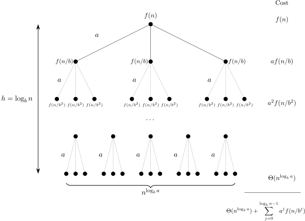
The tree ends at level \(L=\log_b n\) and has \(a^L=n^{\log_b a}\) leaves. The non-leaf levels are numbered \(0,\ldots,L-1\), so \(T(n) = \Theta(n^{\log_b a}) + g(n)\), where \(g(n) = \sum_{j = 0}^{L-1} a^{j} f(n / b^{j})\).
In the first case, \(f(n) = O(n^{\log_b a-\epsilon})\), so \(g(n) = O(n^{\log_b a})\).
In the second case, the cost of the root node already gives \(T(n)=\Omega(f(n))\). By the regularity condition, as long as the subproblems are still large enough, the total cost of level \(j\) is at most \(c^j f(n)\), and these levels cost \(O(f(n))\) altogether. The remaining constant number of levels at the bottom, together with the leaves, cost \(O(n^{\log_b a})=O(f(n))\) in total, so \(T(n)=\Theta(f(n))\).
In the third case, let \(p=\log_b a\). For subproblems that are large enough, the total cost of level \(j\) is \(\Theta(n^p(L-j)^k)\), where \(k\ge0\) is a fixed constant. Pick a fixed \(r_0\ge1\) such that \(b^{r_0}\) reaches that size. Since \(\sum_{r=r_0}^L r^k=\Theta(L^{k+1})\), these levels cost \(\Theta(n^p\log^{k+1}n)\) in total. The remaining constant number of levels at the bottom, together with the leaves, cost \(O(n^p)\) in total; adding this gives the result.
A few examples show how to use the master theorem.
-
\(T(n) = 2T\left(\dfrac{n}{2}\right) + 1\). Here \(a=2, b=2, {\log_2 2} = 1\), and \(\epsilon\) can be any value in \((0, 1]\), so the first case applies and \(T(n) = \Theta(n)\).
-
\(T(n) = T\left(\dfrac{n}{2}\right) + n\). Here \(a=1, b=2, {\log_2 1} = 0\), and \(\epsilon\) can be any value in \((0, 1]\), so the second case applies and \(T(n) = \Theta(n)\).
-
\(T(n) = T\left(\dfrac{n}{2}\right) + {\log n}\). Here \(a=1, b=2, {\log_2 1}=0\), and \(k\) can be taken to be \(1\), so the third case applies and \(T(n) = \Theta(\log^2 n)\).
-
\(T(n) = T\left(\dfrac{n}{2}\right) + 1\). Here \(a=1, b=2, {\log_2 1} = 0\), and \(k\) can be taken to be \(0\), so the third case applies and \(T(n) = \Theta(\log n)\).
Amortized complexity
See amortized complexity for details.
Space complexity
Similarly, space complexity measures how the space an algorithm uses changes with the input size.
Computational complexity
This article has introduced complexity mainly from the viewpoint of algorithm analysis. If you are interested, see computational complexity to go deeper.
This page is an unofficial English translation of the original OI Wiki page (revision b469442a), machine-translated by Claude Fable 5.2 on 2026-11-16. It has been modified from the original by translation and may contain errors. It is not endorsed by OI Wiki.
Found a translation problem? Report it on GitHub.
Authors of the original page: linehk, persdre, Great-designer, Backl1ght, ouuan, ksyx, iamtwz, isdanni, sshwy, Konano, 24OI-bot, Enter-tainer, CCXXXI, Enonya, shuzhouliu, zirnc, chinggg, YHN-ice, Menci, aquastripe, onelittlechildawa, shawlleyw, nullnan, he-zhiyuan, Tiphereth-A, yyyu-star, c-forrest, lailai0916 (full contribution history)
All content on this page is provided under the terms of CC BY-SA 4.0 and SATA; additional terms may apply.