Splay Tree
This page gives a brief introduction to maintaining a binary search tree with a splay tree.
Definition
A splay tree is a balanced binary search tree. Its splay operation keeps rotating some node up to the root while preserving the binary search tree property, and this lets the tree insert, find and delete in amortized \(O(\log n)\) time.1
The splay tree was invented by Daniel Sleator and Robert Tarjan in 1985.
Basic structure and operations
This section covers the basic structure of a splay tree and its core operations, the most important of which is the splay operation.
A splay tree is a binary search tree: for every node, the value of any node in its left subtree \(<\) the value of the node itself \(<\) the value of any node in its right subtree.
Stored information
This article implements the splay tree with arrays in place of pointers. The following information is maintained:
| rt | id | fa[i] | ch[i][0/1] | val[i] | cnt[i] | sz[i] |
|---|---|---|---|---|---|---|
| index of the root | number of nodes in use | parent | indices of the left and right children | value of the node | number of times the value occurs | subtree size |
To initialize, set everything to zero.
Helper operations
We start with a few simple helpers:
dir(x): tells whether node \(x\) is the left or the right child of its parent;push_up(x): after nodes have changed position, recomputes the information of node \(x\) from its children.
Implementation
1 2 3 | |
Rotation
A splay tree is kept balanced by rotations. A rotation moves a node up by one level.
A rotation must guarantee that:
- the inorder traversal of the whole splay tree is unchanged (the binary search tree property must not be broken);
- the information maintained in the affected nodes is still correct;
rtpoints to the root after the rotation.
A splay tree has two kinds of rotation: the left rotation and the right rotation.
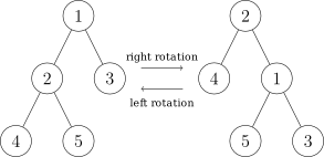
As the figure shows, when a rotation moves a node \(x\) up (\(1\) in the left rotation, \(2\) in the right rotation), its direction is determined entirely by whether \(x\) is the left or the right child of its parent. So the rotation function needs only one argument: the node \(x\) to move up.
The steps of a rotation in detail (let \(x\) be the node to move up, and take the right rotation as the example):
- Record the parent \(y\) of node \(x\) and the parent \(z\) of \(y\) (which may be null), and record whether \(x\) is the left or the right child of \(y\);
- Going bottom-up in the tree as it will be after the rotation, set the left child of \(y\) to the right child of \(x\), the right child of \(x\) to \(y\), and, if \(z\) is not null, the child of \(z\) to \(x\);
- In the same order, set the parent of the current left child of \(y\) (if there is one) to \(y\), the parent of \(y\) to \(x\), and the parent of \(x\) to \(z\);
- Update the node information from the bottom up.
Implementation
1 2 3 4 5 6 7 8 9 10 11 12 | |
In every function you implement, take care never to modify the information of node \(0\).
The splay operation
A splay tree requires that every time a node \(x\) is accessed, it is rotated all the way to the root. This is called the splay operation.
Let \(x\) be the node just accessed. Splaying \(x\) means applying a sequence of splaying steps to it, each of which brings \(x\) closer to the root. Let \(p\) be the parent of \(x\). There are three kinds of splaying step:
-
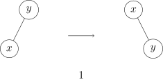
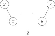
zig: done when \(p\) is the root. The tree is rotated on the edge between \(x\) and \(p\). The zig step exists to deal with the parity of the depth: it is done only as the last step of a splay operation, and only when \(x\) has odd depth at the start of the operation.
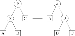
That is, \(x\) is simply rotated right or left (Figures 1 and 2).
-
zig-zig: done when \(p\) is not the root and \(x\) and \(p\) are both right children or both left children. The figure below shows the case where both are left children. The tree is first rotated on the edge joining \(p\) to its parent \(g\), then on the edge joining \(x\) to \(p\).
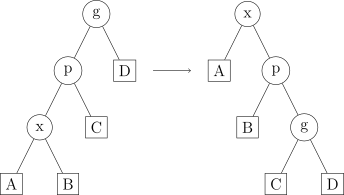
That is, first rotate \(p\) right or left, then rotate \(x\) right or left (Figures 3 and 4).
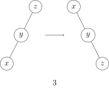
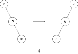
-
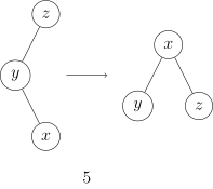
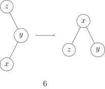
zig-zag: done when \(p\) is not the root and one of \(x\) and \(p\) is a right child while the other is a left child. The tree is first rotated on the edge between \(p\) and \(x\), then on the new edge between \(x\) and \(g\) that this creates.
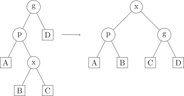
That is, rotate \(x\) left and then right, or right and then left (Figures 5 and 6).
Tip
Work through all \(6\) rotation cases by hand to understand the basic idea of the splay operation.
Comparing the three splaying steps, we see that choosing the right one comes down to two tests: whether \(x\) is a child of the root, and whether \(x\) and its parent are on the same side of their respective parents.
The implementation given here takes an arbitrary root \(z\) and moves any node \(x\) of its subtree up to the position of \(z\):
- Record the parent \(w\) of the root \(z\), so that
fa[x] == wtells us that \(x\) is already at the root; - Record the current parent \(y\) of \(x\). If \(y\) equals \(w\), then \(x\) has reached the root;
- Otherwise, use
fa[y] == wto test whether \(y\) is the root. If it is, a single zig rotates \(x\). If it is not,dir(x) == dir(y)decides between zig-zig and zig-zag: the former rotates \(y\) and then \(x\), the latter rotates \(x\) twice.
Implementation
1 2 3 4 5 6 7 | |
The splay operation is the heart of the splay tree, and it is what guarantees the time complexity. Whenever you walk down the tree to a node, make sure you splay afterwards.
The splay operation also recomputes, from the bottom up, the information of every node on the path from the current node \(x\) to the root \(z\). This is exactly why we can modify a node that is not the root and then splay it up to the root to bring the information of the whole tree up to date.
Time complexity
Performing \(m\) splay operations on a splay tree of size \(n\) takes \(O((m+n)\log n)\) time, which is \(O(\log n)\) amortized per operation.
Proof of complexity by the potential method
It suffices to analyze the cost of the three steps zig, zig-zig and zig-zag. We use the potential method, which derives the amortized cost of an operation from the change in potential. Suppose \(m\) splay operations are performed on a splay tree with \(n\) nodes. The analysis goes as follows:
Definitions:
- Potential of a single node: \(w(x) = \log(\text{size}(x))\), where \(\text{size}(x)\) is the size of the subtree rooted at node \(x\).
- Potential of the whole tree: \(\varphi = \sum w(x)\), the sum of the potentials of all nodes in the tree. The initial potential satisfies \(\varphi_0 \leq n \log n\).
- Amortized cost of the \(i\)-th operation: \(c_i = t_i + \varphi_i - \varphi_{i-1}\), where \(t_i\) is the actual cost of the operation, and \(\varphi_i\) and \(\varphi_{i-1}\) are the potentials after and before it.
Properties:
-
If \(p\) is the parent of \(x\), then \(w(p) \geq w(x)\): the potential of a parent is no less than that of its child.
-
The subtree size of the root is the same before and after an operation, so the potential of the root does not change during the operation.
-
If \(\text{size}(p)\ge\text{size}(x)+\text{size}(y)\), then \(2w(p) - w(x) - w(y) \geq 2\).
Proof of property 3
By the AM-GM inequality,
Next we analyze the potential for the zig, zig-zig and zig-zag steps in turn. Let \(w(x)\) and \(w'(x)\) be the potentials of node \(x\) before and after the step. The nodes are named as above.
zig: By properties 1 and 2, \(w(p) = w'(x)\) and \(w'(x) \geq w'(p)\). The amortized cost is therefore
zig-zig: By properties 1 and 2, \(w(g) = w'(x)\), \(w'(x) \geq w'(p)\) and \(w(x) \leq w(p)\). Since
property 3 gives
The amortized cost is therefore
zig-zag: By properties 1 and 2, \(w(g) = w'(x)\) and \(w(p) \geq w(x)\). Since \(\text{size}'(x)>\text{size}'(p)+\text{size}'(g)\), property 3 gives
The amortized cost is therefore
A single splay operation:
Let \(w^{(j)}(x)=(w^{(j-1)})'(x)\) and \(w^{(0)}(x)=w(x)\). Suppose a splay operation consists of \(k\) splaying steps and ends with node \(x_{1}\) at the root. It is made up of some number of zig-zig and zig-zag steps and at most one zig step. Each step of the first two kinds has amortized cost at most \(3(w'(x)-w(x))\), and the last step has amortized cost at most \(3(w'(x) - w(x))+1\), so the total amortized cost is at most
Hence a splay operation has amortized complexity \(O(\log n)\), and so do the operations built on it, such as insertion, query and deletion.
Conclusion:
After \(m\) splay operations, the actual cost satisfies
So \(m\) splay operations take \(O((m+n)\log n)\) actual time.
Why does rebalancing in a splay tree achieve \(O(\log n)\) amortized complexity?
The naive way to rebalance is to rotate the node up again and again until it becomes the root. The trouble is that on a chain-shaped tree in which every child is a left (or right) child, this amounts to one zig step after another, so the constant term \(1\) in the amortized cost of zig keeps accumulating and the amortized complexity reaches the order of \(O(n)\). Rebalancing in a splay tree is designed to avoid this accumulation of constants over consecutive zig steps: a complete splay operation performs at most one lone zig, and that is what improves the time complexity.
Balanced tree operations
This section shows how to implement the common balanced tree operations on a splay tree. The most important are finding an element by value and by rank: each locates a particular element and moves it up to the root, ready for further processing.
As an example, this section works through the template problem Ordinary Balanced Tree.
Finding by value
Since this is a binary search tree, the node with a given value \(v\) can be found simply by comparing \(v\) with the value of the current node on the way down. Once found, the element is moved up to the root.
Bear in mind that the tree often contains no such node. In that case, record the last node visited (\(y\) in the implementation) and move \(y\) up to the root. The value stored at \(y\) is then either the largest element less than \(v\) (the predecessor of \(v\)) or the smallest element greater than \(v\) (the successor of \(v\)). This is because the search guarantees that the left subtree always holds the values less than \(v\) and the right subtree the values greater than \(v\).
Implementation
1 2 3 4 5 | |
This implementation lets you choose any node \(z\) as the root and search by value within its subtree.
Access by rank
Because subtree sizes are stored, a splay tree can also access an element by rank, that is, find the \(k\)-th smallest element of the tree.
Let \(k\) be the remaining rank. The steps are:
- If the left subtree is nonempty and the remaining rank \(k\) is at most its size, search in the left subtree;
- otherwise, if \(k\) is at most the size of the left subtree plus the number of occurrences of the root's value, the root is the node we are looking for;
- otherwise, subtract from \(k\) the size of the left subtree plus the number of occurrences of the root's value, and continue in the right subtree;
- finally, move the element found up to the root.
Implementation
1 2 3 4 5 6 7 8 9 10 11 12 13 14 | |
This implementation requires that the rank \(k\) does not exceed the size of the tree rooted at \(z\).
Operation \(4\) of the template problem asks for the value with a given rank: call this function and return the value.
Implementation
1 2 3 4 5 | |
Merging
Sometimes two splay trees have to be merged.
Let \(x\) and \(y\) be the roots of the two trees. For the result to be a binary search tree, the maximum of tree \(x\) must be less than the minimum of tree \(y\). This condition usually holds, because the two trees tend to have been split off from a larger subtree.
To merge:
- If \(x\) or \(y\) or both are empty trees, return the root of the nonempty one, or the empty tree;
- otherwise, call
loc(y, 1)to move the minimum of tree \(y\) up to the root \(y\), set its left child (which must be empty at this point) to \(x\), update the node information, and return node \(y\).
Implementation
1 2 3 4 5 6 7 8 | |
Splitting is similar. A splay tree can therefore do everything the way a non-rotating treap does, range operations included. Below we present a way of handling range operations that is more in the style of a splay tree.
Insertion
Insertion is a fairly involved procedure. The steps are as follows (let \(v\) be the value to insert):
- As when finding by value, walk down by \(v\) to the node storing \(v\) or to an empty node, recording the parent \(y\) on the way;
- if a node \(x\) storing \(v\) exists, update its information; otherwise create a new node \(x\);
- splay, moving the last node \(x\) up to the root.
Implementation
1 2 3 4 5 6 7 8 9 10 11 12 13 14 15 | |
This implementation can insert directly into an empty tree. If you would rather not handle the empty tree, insert dummy nodes into the tree beforehand.
Deletion
Deletion is also a fairly involved operation. The steps are as follows (let \(v\) be the value to delete):
- First find the node storing the value \(v\) and move it up to the root;
- if no node stores it, return (the previous step has already splayed);
- otherwise, update the node information;
- if the number of occurrences of the root's value has dropped to zero, delete the node: merge its left and right subtrees and make the result the new root. Before merging, set the parents of the roots of the two subtrees to null.
Implementation
1 2 3 4 5 6 7 8 9 10 11 12 13 | |
Rank query
Access the node by the value \(v\) (moving it up to the root), then return the corresponding rank.
Note that when \(v\) is not in the tree, the root that find(rt, v) leaves behind may be either smaller or larger than \(v\), and the two cases must be handled separately.
Implementation
1 2 3 4 | |
Predecessor query
The predecessor is the largest number less than \(v\). The steps are:
- Access the node by the value \(v\) (moving it up to the root);
- if the value at the root is less than \(v\), it must be the largest such value, so return it;
- otherwise, find the maximum of the left subtree and move it up to the root.
The last step is equivalent to calling loc(ch[rt][0], sz[ch[rt][0]]) directly, only without the unnecessary checks.
Implementation
1 2 3 4 5 6 7 8 9 | |
This implementation allows for a predecessor that does not exist, in which case it returns \(-1\).
Successor query
The successor is the smallest number greater than \(v\). It is found in the same way as the predecessor, except that the maximum of the left subtree is replaced by the minimum of the right subtree, that is, by a call to loc(ch[rt][1], 1).
Implementation
1 2 3 4 5 6 7 8 9 | |
Reference implementation
To close this section, here is a reference implementation for the template problem Ordinary Balanced Tree.
Reference implementation
1 2 3 4 5 6 7 8 9 10 11 12 13 14 15 16 17 18 19 20 21 22 23 24 25 26 27 28 29 30 31 32 33 34 35 36 37 38 39 40 41 42 43 44 45 46 47 48 49 50 51 52 53 54 55 56 57 58 59 60 61 62 63 64 65 66 67 68 69 70 71 72 73 74 75 76 77 78 79 80 81 82 83 84 85 86 87 88 89 90 91 92 93 94 95 96 97 98 99 100 101 102 103 104 105 106 107 108 109 110 111 112 113 114 115 116 117 118 119 120 121 122 123 124 125 126 127 128 129 130 131 132 133 134 135 136 137 138 139 140 141 142 143 144 145 146 147 148 149 150 151 | |
Sequence operations
A splay tree can also be used on a sequence, to maintain range information. Compared with a segment tree, a splay tree has a larger constant factor but supports more complex sequence operations, such as range reversal. As mentioned above, a splay tree also supports splitting and merging, so it can imitate a non-rotating treap to perform range operations; we do not go into that here. This section is about implementing range operations with the splay operation.
A splay tree built from a sequence has the following properties:
- its inorder traversal is the original sequence read from left to right;
- a node of the splay tree represents one element of the original sequence;
- a subtree of the splay tree represents a range of the original sequence.
Thanks to the splay operation, the splay subtree that represents a given range can be extracted quickly.
As an example, this section works through the template problem Artistic Balanced Tree.
Building the tree from a sequence
Before any operation, the splay tree has to be built from the given sequence. Given how a splay tree behaves, it is enough to build a chain in which every node has only a left child. This takes \(O(n)\) time.
Reference implementation
1 2 3 4 5 6 7 8 9 10 | |
The splay operation at the end updates the node information from the bottom up. To make the range operations below easier, a sentinel node is added at each end of the sequence.
Range reversal
Range reversal shows how range operations work (let the range be \([L,R]\)):
- First move node \(L-1\) up to the root; then, inside its right subtree, move node \(R+1\) up to the root of that subtree;
- now let \(x\) be the left child of the right child of the root: the subtree rooted at \(x\) corresponds to the range \([L,R]\);
- apply the operation for the range \([L,R]\) at \(x\) and set the lazy tag;
- push the tag down once at \(x\), then splay \(x\) up to the root.
The first step needs exactly the "access by rank" operation from the balanced tree operations above, because the label of an element is its rank. Since lazy tags now have to be managed, its implementation differs slightly from the one above.
Reference implementation
1 2 3 4 5 6 7 8 | |
The splay operation in the last step is not there to guarantee the complexity, but to update the node information. Because splaying involves the left and right children of node \(x\), the tag at \(x\) has to be pushed down once beforehand. Of course, for range reversal alone, reversing a subrange has no effect on the ancestors, so leaving this step out would also be correct. The implementation keeps these two lines to show what to do in the general case.
Managing lazy tags
First we need the helper functions lazy_reverse(x) and push_down(x). The former swaps the left and right children and updates the lazy tag; the latter pushes the tag down.
Reference implementation
1 2 3 4 5 6 7 8 9 10 11 12 | |
After that, all we have to do is push tags down whenever we pass through a node on the way down. The template problem asks for little: only the search by rank (loc) walks down the tree. Note that the tag must be pushed down before the function visits each new node.
Reference implementation
1 2 3 4 5 6 7 8 9 10 11 12 | |
Walking down has already removed every lazy tag on the path, so no tags need handling when the splay operation moves a node up. But take care with the node on which the range operation was performed: it too lies on the path of the splay operation, and since it has only just been operated on, it may carry a tag that has not been pushed down. Push that tag down first and then splay, exactly as we did above.
Reference implementation
To close this section, here is a reference implementation for the template problem Artistic Balanced Tree.
Reference implementation
1 2 3 4 5 6 7 8 9 10 11 12 13 14 15 16 17 18 19 20 21 22 23 24 25 26 27 28 29 30 31 32 33 34 35 36 37 38 39 40 41 42 43 44 45 46 47 48 49 50 51 52 53 54 55 56 57 58 59 60 61 62 63 64 65 66 67 68 69 70 71 72 73 74 75 76 77 78 79 80 81 82 83 84 85 86 87 88 89 90 91 92 93 94 95 96 97 98 99 100 101 102 103 | |
Practice problems
These problems are all straightforward uses of a splay tree as a binary search tree:
- [Template] Ordinary Balanced Tree
- [Template] Artistic Balanced Tree
- [HNOI2002] Turnover Statistics
- [HNOI2004] Pet Adoption Center
Splay trees also appear in more complex settings:
- [Cerc2007] Robotic Sort
- [HNOI2011] Bracket Repair / [JSOI2011] Bracket Sequence
- Silly Balanced Tree (Nested Trees)
- BZOJ 2827 No Bird Flies over a Thousand Mountains
- [Lydsy1706 Monthly Contest] K-th Smallest Query
- POJ3580 SuperMemo
References and notes
Parts of this article are drawn from the algocode algorithms blog. Special thanks!
-
A splay tree only guarantees an amortized complexity of \(O(\log n)\). It does not maintain a balance condition the way an AVL tree or a red–black tree does, and it may even degenerate into a chain after a sequence of operations. A single operation therefore takes \(O(n)\) in the worst case. ↩
This page is an unofficial English translation of the original OI Wiki page (revision 89bae42e), machine-translated by Claude Fable 5.2 on 2026-11-16. It has been modified from the original by translation and may contain errors. It is not endorsed by OI Wiki.
Found a translation problem? Report it on GitHub.
Authors of the original page: Ir1d, hsfzLZH1, Xeonacid, abc1763613206, 24OI-bot, longlongzhu123, partychicken, GavinZhengOI, Catreap, ouuan, hly1204, StudyingFather, countercurrent-time, Henry-ZHR, sshwy, ezoixx130, Gesrua, Alpacabla, NachtgeistW, H-J-Granger, Enter-tainer, mcendu, xiaolaohuqwq, ksyx, Macesuted, iamtwz, isdanni, Tiphereth-A, Great-designer, Persdre, shuzhouliu, CoelacanthusHex, aofall, Marcythm, GrapeLemonade, yuhuoji, zzxLLLL, Early0v0, xiaofu-15191, yyyu-star, HeRaNO, Molmin, c-forrest, zcz0263, not-exist (full contribution history)
All content on this page is provided under the terms of CC BY-SA 4.0 and SATA; additional terms may apply.