CDQ Divide and Conquer
This page introduces CDQ divide and conquer.
Overview
CDQ divide and conquer is an idea rather than a specific algorithm, much like dynamic programming. The idea has by now been extended very widely. Depending on the principle and on how the code is written, its uses fall roughly into three classes:
- Solving problems about pairs of points.
- Optimizing and computing the transitions of 1D dynamic programming.
- Using CDQ divide and conquer to turn certain dynamic problems into static ones.
The idea was first written up and summarized by Danqi Chen, an IOI 2008 gold medalist, while she was in high school, and it is named after her.1
Problems about pairs of points
Most problems of this kind look like "given a sequence of length \(n\), count the pairs \((i,j)\) that have some property" or "given a sequence of length \(n\), find a pair \((i,j)\) that maximizes some function".
CDQ divide and conquer solves such problems as follows:
-
Find the midpoint \(mid\) of the sequence.
-
Partition all pairs \((i,j)\) into three classes:
- pairs with \(1 \leq i \leq mid,1 \leq j \leq mid\);
- pairs with \(1 \leq i \leq mid ,mid+1 \leq j \leq n\);
- pairs with \(mid+1 \leq i \leq n,mid+1 \leq j \leq n\).
-
Split the sequence \((1,n)\) into the two sequences \((1,mid)\) and \((mid+1,n)\). Every pair of the first or third class now lies inside one of these two sequences.
-
Handle these two classes of pairs recursively.
-
Find a way to handle the pairs of the second class.
The idea of CDQ divide and conquer, then, is to keep handing pairs down to the left and right ranges by recursion.
In practice we usually write a function solve(l,r) that handles the pairs with \(l \leq i \leq r,l \leq j \leq r\). The recursive part of the procedure above is then just the calls solve(l,mid) and solve(mid+1,r). The remaining pairs, those of the second class, need an algorithm designed separately.
Example problems
3D Partial Order
Given a sequence in which every point has three attributes \(a_i,b_i,c_i\), count the pairs \((i,j)\) in the sequence with \(a_j \leq a_i\), \(b_j \leq b_i\), \(c_j \leq c_i\) and \(j \ne i\).
Approach
3D partial order is the classic problem for CDQ divide and conquer.
The problem asks us to count pairs in a sequence, so let us try CDQ divide and conquer.
First sort the sequence by \(a\).
Suppose we are writing solve(l,r) and the recursive calls solve(l,mid) and solve(mid+1,r) have done their part. What remains is to count, among the pairs \((i,j)\) with \(l \leq i \leq mid\) and \(mid+1 \leq j \leq r\), those that also satisfy the constraints \(a_{i} \leq a_{j}\), \(b_{i} \leq b_{j}\) and \(c_{i} \leq c_{j}\).
A moment's thought shows that the constraint \(a_{i} \leq a_{j}\) no longer matters: \(i\) is at most \(mid\) and \(j\) is greater than \(mid\), so \(i\) is certainly less than \(j\), and since the sequence is sorted by \(a\) we must have \(a_{i} \leq a_{j}\). Two constraints remain: \(b_{i} \leq b_{j}\) and \(c_{i} \leq c_{j}\). Using them, we can enumerate \(j\) and count the \(i\) that satisfy both.
To make the enumeration easy, sort the points in \((l,mid)\) and the points in \((mid+1,r)\) by \(b\) in increasing order. Then enumerate the \(j\) one by one, inserting every point \(i\) with \(b_{i} \leq b_{j}\) into some data structure (here we choose a Fenwick tree). Now ask the Fenwick tree how many of its points have a \(c\) value less than or equal to \(c_{j}\): that is the number of \(i\) that form a valid pair with this point \(j\).
To insert a point whose \(c\) value equals \(x\), add one at position \(x\) of the Fenwick tree. Asking how many points in the Fenwick tree are less than or equal to \(x\) is then just a prefix sum query. As long as we apply coordinate compression to all the \(c\) values beforehand, the complexity is right.
For every \(j\) we have to insert all points \(i\) with \(b_{i} \leq b_{j}\) into the Fenwick tree. All the \(i\) and all the \(j\) are already sorted by \(b\), so if we insert the points with two pointers, the number of insertions into the Fenwick tree drops from \(O(n^2)\) to \(O(n)\).
This procedure handles the pairs of the second class in \(O(n\log n)\) time. The running time of the algorithm is then \(T(n)=T(\lfloor \frac{n}{2} \rfloor)+T(\lceil \frac{n}{2} \rceil)+O(n\log n)=O(n\log^2n)\).
Example code
1 2 3 4 5 6 7 8 9 10 11 12 13 14 15 16 17 18 19 20 21 22 23 24 25 26 27 28 29 30 31 32 33 34 35 36 37 38 39 40 41 42 43 44 45 46 47 48 49 50 51 52 53 54 55 56 57 58 59 60 61 62 63 64 65 66 67 68 69 70 71 72 73 74 75 76 77 78 79 80 81 82 83 84 85 86 87 88 89 90 91 92 93 94 95 96 97 98 99 100 101 102 103 104 105 | |
CQOI2011 Dynamic Inversions
The number of inversions of a sequence \(a\) is defined as the number of elements of the set \(\{(i,j)| i < j \wedge a_i > a_j \}\).
You are given a permutation of \(1\sim n\), from which \(m\) elements are deleted one after another in a given order. Your task is to count the inversions of the whole sequence before each deletion.
Example code
1 2 3 4 5 6 7 8 9 10 11 12 13 14 15 16 17 18 19 20 21 22 23 24 25 26 27 28 29 30 31 32 33 34 35 36 37 38 39 40 41 42 43 44 45 46 47 48 49 50 51 52 53 54 55 56 57 58 59 60 61 62 63 64 65 66 67 68 69 70 71 72 73 74 75 76 77 78 79 80 81 82 83 84 85 86 87 88 89 90 91 92 93 94 95 96 97 98 99 100 101 102 103 104 105 106 107 108 109 110 111 112 113 114 115 116 117 118 119 | |
Optimizing 1D/1D DP transitions with CDQ divide and conquer
Related content: optimizing DP with CDQ divide and conquer
1D/1D dynamic programming is a particular class of DP problems in which the DP array is one-dimensional and a transition takes \(O(n)\). When conditions are favorable, CDQ divide and conquer can sometimes bring their running time down from \(O(n^2)\) to \(O(n\log^2n)\).
For example, take a sequence in which every element has two attributes, \(a\) and \(b\). We want to evaluate a DP with the following recurrence:
\(dp_{i}=1+ \max_{j=1}^{i-1}dp_{j}[a_{j} < a_{i}][b_{j} < b_{i}]\)
This is the recurrence for a 2D longest increasing subsequence: only the points \(j\) with \(j < i,a_{j} < a_{i},b_{j} < b_{i}\) can update the DP value of point \(i\).
Computing the transitions directly clearly takes \(O(n^2)\). Here is how CDQ divide and conquer speeds them up.
A transition from \(dp_{j}\) to \(dp_{i}\) is also a relation between a pair of points, so we treat it much as CDQ divide and conquer treats pairs of points.
The procedure is fairly routine. Suppose the range being processed is \((l,r)\). The algorithm goes roughly as follows:
- If \(l=r\), the \(\max\) part of \(dp_{r}\) has already been computed: set \(dp_{r} \gets dp_{r} + 1\) and return.
- Call
solve(l,mid)recursively. - Handle all transitions with \(l \leq j \leq mid\) and \(mid+1 \leq i \leq r\).
- Call
solve(mid+1,r)recursively.
Step 3 works much like solving 3D partial order with CDQ divide and conquer. For the transitions with \(l \leq j \leq mid\) and \(mid+1 \leq i \leq r\), the constraint \(j < i\) no longer needs any attention. So, as before, we sort all the points \(i\) and all the points \(j\) by \(a\), insert the points \(j\) into a Fenwick tree with two pointers, and query the prefix maximum to update \(dp_{i}\).
Proof of correctness of the transitions
The biggest difference between this way of writing CDQ and the one for relations between pairs of points lies in the step that handles the pairs with \(l \leq j \leq mid\) and \(mid+1 \leq i \leq r\). In the version for pairs of points, this step can go anywhere. When CDQ divide and conquer optimizes a DP, however, it has to sit between \(solve(l,mid)\) and \(solve(mid+1,r)\). The reason is that the transitions of a DP are ordered. They must satisfy two conditions, or the result is wrong:
-
Every \(dp_{j}\) used to compute \(dp_{i}\) must already be fully computed; no half-finished value is allowed.
-
Every \(dp_{j}\) that is meant to be used in computing \(dp_{i}\) must actually update \(dp_{i}\); none may be left out.
The \(O(n^2)\) brute force satisfies both conditions easily. With CDQ divide and conquer, though, the order of the transitions is clearly scrambled, so their correctness has to be examined.
The recursion tree of CDQ divide and conquer is shown below.
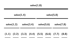
Run the algorithm above and take point \(8\) as an example. Its DP value is updated in three calls, solve(1,8), solve(5,8) and solve(7,8), and the points that update it in these three calls form the three disjoint ranges \((1,4)\), \((5,6)\) and \((7,7)\). Now take point \(5\): its DP value is settled in the call solve(1,8), and the range that updates it is \((1,4)\). Look closely and you will see that the DP value of a point \(i\) is updated \(\log\) times, and that the ranges updating it are exactly the \(\log\) ranges into which a segment tree splits \((1,i-1)\). So every valid \(j\) really does update point \(i\), and condition 2 holds.
Next, trace how the algorithm executes:
- The first call to finish is
solve(1,1). At this point \(dp_{1}\) is fully computed. - The first call to perform its transitions is
solve(1,2). At this point \(dp_{2}\) has received all its transitions. - The second call to finish is
solve(2,2). At this point \(dp_{2}\) is fully computed. - Then
solve(1,2)finishes, and all the \(dp\) values in the range \((1,2)\) are computed. - The next call to perform its transitions is
solve(1,4). Once they are done, \(dp_{3}\) has received all its transitions. - The next call to finish is
solve(3,3), and \(dp_{3}\) is now fully computed. - The next transitions are those of
solve(3,4). \(dp_{4}\) was updated once from \((1,2)\) insolve(1,4)and is now updated from \((3,3)\), so it too has received all its transitions. solve(4,4)finishes, and \(dp_{4}\) is fully computed.solve(3,4)finishes, and the values in \((3,4)\) are fully computed.solve(1,4)finishes, and the values in \((1,4)\) are fully computed.- ...
Simulating the calls shows one thing: whenever solve(l,r) finishes, all DP values in the range \((l,r)\) are fully computed. Whenever we perform the transitions, solve(l,mid) has already finished, so every transition we perform is valid, and condition 1 holds.
The trace also shows that if we view the recursion tree of CDQ divide and conquer as a segment tree, then CDQ divide and conquer is an inorder traversal of that segment tree. In effect we process all the DP values in order, and only the transitions are split up. So the algorithm is correct.
Example problems
SDOI2011 Missile Interception
To defend itself against missile attacks from an enemy country, a country has developed a missile interception system. The system has a flaw, however: its first shell can reach any height and intercept a missile of any speed, but every later shell can go no higher than the one before it, and the missile it intercepts can fly no faster than the one intercepted before. One day the radar picks up incoming enemy missiles. The system is still in its trial phase, so there is only one of it, and it may not be able to intercept all the missiles.
When not all the missiles can be intercepted, we of course choose a plan that minimizes the country's losses, that is, one that intercepts as many missiles as possible. There may be more than one such plan. If there are several optimal plans, we pick one of them at random as the final blueprint for the interception.
Our spies have obtained the heights and speeds of all the enemy missiles. Your task is to compute, for each missile, the probability that it is intercepted when the decision above is carried out.
Example code
1 2 3 4 5 6 7 8 9 10 11 12 13 14 15 16 17 18 19 20 21 22 23 24 25 26 27 28 29 30 31 32 33 34 35 36 37 38 39 40 41 42 43 44 45 46 47 48 49 50 51 52 53 54 55 56 57 58 59 60 61 62 63 64 65 66 67 68 69 70 71 72 73 74 75 76 77 78 79 80 81 82 83 84 85 86 87 88 89 90 91 92 93 94 95 96 97 98 99 100 101 102 103 104 105 106 107 108 109 110 111 112 113 114 115 116 117 118 119 120 121 122 123 124 125 126 127 128 129 130 131 132 133 134 135 136 137 138 139 140 141 142 143 144 145 146 147 148 149 150 151 152 153 154 155 156 157 158 159 160 161 162 163 164 165 166 167 | |
Turning dynamic problems into static ones
In the first two settings, CDQ divide and conquer halves a sequence and handles the relations between pairs of points recursively in order to get a good complexity. In this section, what gets halved is not an ordinary sequence but the timeline.
This applies to data structure problems of the form "support such-and-such updates and then answer such-and-such queries". Problems of this kind have two features:
- If the queries are taken offline, all the operations naturally line up in a sequence ordered by time.
- Every update is closely tied to the queries that come after it, and there are \(O(n^2)\) such update-query pairs in total.
We can run CDQ divide and conquer on this sequence of operations to handle the relations between updates and queries.
As in CDQ divide and conquer on pairs of points, suppose the sequence being divided is \((l,r)\). We first recursively handle the update-query pairs within \((l,mid)\) and within \((mid+1,r)\), and then all the update-query pairs with \(l \leq i \leq mid\) and \(mid+1 \leq j \leq r\), where \(i\) is an update and \(j\) is a query.
Note that if the updates are independent of one another (ordinary addition and subtraction, for example), it does not matter in which order we run the three steps: solve(l,mid), solve(mid+1,r), and the handling of the pairs with \(l \leq i \leq mid\) and \(mid+1 \leq j \leq r\). If the updates are not independent (assignments, say), what the sequence looks like after an update may depend on what it looked like before. The step that handles all the update-query pairs crossing mid must then go between solve(l,mid) and solve(mid+1,r). The reason is the same as for optimizing 1D/1D dynamic programming with CDQ divide and conquer: only by dividing in inorder traversal order can we guarantee that every update is applied strictly in chronological order.
Example problems
Rectangle addition, rectangle sum
Maintain a 2D array that supports adding a number to every cell of a rectangular region and querying the sum over a rectangular region.
Approach
The version of this problem without updates, "given a 2D array, answer many queries for the sum over a rectangular region", has a classic solution that combines a sweep line with a segment tree. Split each rectangle into two operations, an insertion and a deletion, then write each query as a difference of 2D prefix sums, and finally process everything offline. The original problem has updates, though, so this solution cannot be used directly.
Let us try CDQ divide and conquer on it. Take all the queries and updates offline. These operations form a sequence, and there are \(O(N^2)\) update-query pairs. Follow the general procedure of CDQ divide and conquer again: partition all the pairs into three classes, handle only the update-query pairs that cross \(mid\) at this level of the divide and conquer, and leave the remaining ones to the recursion.
Now all the updates are finished before the queries begin. The original problem is then equivalent to "there are some static rectangles in the plane; answer query after query for the sum over a rectangular region".
A sweep line handles all the update-query pairs that cross \(mid\) in \(O(n\log n)\) time. All that is left is to recurse on the update-query pairs of the left side and of the right side.
In CDQ divide and conquer implemented this way, the same query is processed \(O(\log n)\) times. That does not matter, because the sets of updates that contribute to the query each time are disjoint. The whole procedure runs in \(T(n)=T(\lfloor \frac{n}{2} \rfloor)+T(\lceil \frac{n}{2} \rceil)+ O(n\log n)=O(n\log^2n)\).
Look back at this procedure. At the start we could solve only the static rectangle addition, rectangle sum problem, yet simply by applying CDQ divide and conquer we can solve the dynamic one offline. The essence of turning a dynamic problem into a static one is that CDQ divide and conquer handles, each time, only the update-query pairs that cross one particular point, so the only problem we have to think about is the simple one in which every query comes after every update. This is exactly why CDQ divide and conquer is called "a tool for turning dynamic problems into static problems".
[Ynoi2016] Insects in the Mirror
Maintain a sequence \(a_i\) of length \(n\) under \(m\) operations.
- Set the values in the range \([l,r]\) to \(x\).
- Query how many distinct numbers occur in the range \([l,r]\); a number that occurs several times is counted only once.
The problem in one sentence: range assignment, range count of distinct colors.
Approach
For every position, maintain the position of the first point to its left that has the same color, and call it \(pre_{i}\). Counting the colors in a range then becomes a classic 2D point counting problem.
By treating a contiguous stretch of one color as a single point, one can prove that \(pre\) changes \(O(n+m)\) times in total, that is, a single operation causes only \(O(1)\) changes to the values of \(pre\). So we can use CDQ divide and conquer to solve a dynamic problem with point addition and rectangle sum queries.
The actual changes to the \(pre\) array can be worked out with std::set. This trick of maintaining contiguous ranges in a set is also known as the old driver tree.
Example code
1 2 3 4 5 6 7 8 9 10 11 12 13 14 15 16 17 18 19 20 21 22 23 24 25 26 27 28 29 30 31 32 33 34 35 36 37 38 39 40 41 42 43 44 45 46 47 48 49 50 51 52 53 54 55 56 57 58 59 60 61 62 63 64 65 66 67 68 69 70 71 72 73 74 75 76 77 78 79 80 81 82 83 84 85 86 87 88 89 90 91 92 93 94 95 96 97 98 99 100 101 102 103 104 105 106 107 108 109 110 111 112 113 114 115 116 117 118 119 120 121 122 123 124 125 126 127 128 129 130 131 132 133 134 135 136 137 138 139 140 141 142 143 144 145 146 147 148 149 150 151 152 153 154 155 156 157 158 159 160 161 162 163 164 165 166 167 168 169 170 171 172 173 174 175 176 177 178 179 180 181 182 183 184 185 186 187 188 189 190 191 192 193 194 195 196 197 198 199 200 201 202 203 204 205 206 207 208 209 210 211 212 213 214 215 216 217 218 219 220 221 222 223 224 225 226 227 228 229 230 231 232 233 234 235 236 237 238 239 240 | |
[HNOI2010] City Construction
PS is a large country with a great many cities. Its king, Louis, has been racking his brains over the cities' transport network. Louis can build roads between certain pairs of cities, and roads between different pairs of cities cost different amounts to build.
Louis wants to build as few roads as possible so that all the cities in the country are connected. For various reasons, however, the cost of building a road between cities changes over time, and Louis keeps receiving news that the construction cost of some road has changed. After each piece of news he wants to know at once the minimum total cost of connecting the cities. Louis has decided to ask you for help with this task.
The problem in one sentence: given a graph whose edge weights are updated dynamically, output the minimum total cost of its minimum spanning tree after every update.
Approach
This problem can in fact be solved by segment tree divide and conquer combined with a Link Cut Tree, but that implementation has too large a constant factor and may need some clever constant-factor optimization to pass. So let us consider CDQ divide and conquer instead.
Unlike the problems that CDQ divide and conquer usually solves, this one offers no update-query relation to divide on, because we cannot consider in isolation "what updating one edge contributes to the minimum spanning tree of the whole graph". The traditional CDQ divide and conquer approach does not seem to work very well.
The earlier example problems show that ordinary CDQ divide and conquer has a special connection with the segment tree: during CDQ divide and conquer we implicitly build a segment tree (because the recursion tree of CDQ divide and conquer is a segment tree). Ordinary CDQ looks at the relation between the left and right children of a segment tree node. In this problem, what we need to look at is the relation between a parent and its children. In other words, if we can find a way to make the size of the graph in solve(l,r) depend on the length of the range, the problem is solved.
So how, concretely, do we design the algorithm?
Suppose we are constructing the edge set for the minimum spanning tree of the range \((l,r)\), and we know the edge set of its parent's minimum spanning tree. Give the edges that change within the range \((l,r)\) weight \(+ \infty\), then weight \(-\infty\), and run Kruskal's algorithm once for each to find the edges that are in the minimum spanning tree.
For a given edge:
- If it does not appear in the minimum spanning tree in which all the updated edge weights are set to \(+\infty\), it cannot appear in the minimum spanning tree of any of the queries in \((l,r)\). So the only edges we add to the edge set of \((l,r)\) are the tree edges of that minimum spanning tree.
- If it appears in the minimum spanning tree in which all the updated edge weights are set to \(-\infty\), it is certain to appear in the minimum spanning tree throughout the range \((l,r)\). We can then use a disjoint set union to contract the vertices these edges join, and add the weights of these edges to the answer.
This constructs the edge set of the range \((l,r)\). The minimum spanning tree computed from these edges is equivalent to the one computed directly on the original graph.
Why, then, is our complexity right?
First, the updated edges always go into our edge set, and there are \(O(len)\) of them.
Next we have to show that the edge set does not contain too many edges that were not updated. The only ones we add are the tree edges of the minimum spanning tree with all the updated weights set to \(+\infty\), so we add no more edges than the current graph has vertices.
Now it is enough to show that the graph has \(O(len)\) vertices at every level of the recursion; it then follows that it has \(O(len)\) edges.
Showing that the number of vertices is \(O(len)\) is now very easy. Each time we recurse downward, the edges we contract are the edges of the \(-\infty\) spanning tree that were not updated. Seen the other way round, we cut every updated edge that appears in the \(-\infty\) spanning tree. Clearly we cut at most \(len\) edges, so the whole graph splits into at most \(O(len)\) connected components, and the new graph has \(O(len)\) vertices. This proves that every graph we run Kruskal's algorithm on has size \(O(len)\), and hence that each level takes \(O(n\log n)\) time.
The time complexity is \(T(n)=T(\lfloor \frac{n}{2} \rfloor)+T(\lceil \frac{n}{2} \rceil)+ O(n\log n)=O(n\log^2n)\).
The implementation can be a little tricky. Note that the disjoint set union must not use path compression, or it will no longer support rollback. There is also no need to actually carry out the contraction: the Kruskal run at each level can simply work in the disjoint set union of the level above.
Example code
1 2 3 4 5 6 7 8 9 10 11 12 13 14 15 16 17 18 19 20 21 22 23 24 25 26 27 28 29 30 31 32 33 34 35 36 37 38 39 40 41 42 43 44 45 46 47 48 49 50 51 52 53 54 55 56 57 58 59 60 61 62 63 64 65 66 67 68 69 70 71 72 73 74 75 76 77 78 79 80 81 82 83 84 85 86 87 88 89 90 91 92 93 94 95 96 97 98 99 100 101 102 103 104 105 106 107 108 109 110 111 112 113 114 115 116 117 118 119 120 121 122 123 124 125 126 127 128 129 130 131 132 133 134 135 136 137 138 139 140 141 142 143 144 145 146 147 148 149 150 151 152 153 154 155 156 157 158 159 160 161 162 163 164 165 166 167 168 169 170 171 172 173 174 175 176 177 178 179 180 181 182 183 184 185 186 187 188 189 190 191 192 193 194 195 196 197 198 199 200 201 202 203 204 205 206 207 208 209 210 211 212 213 214 215 216 217 218 219 220 221 222 223 224 225 226 | |
References and notes
This page is an unofficial English translation of the original OI Wiki page (revision 9bb3a8e6), machine-translated by Claude Fable 5.2 on 2026-11-16. It has been modified from the original by translation and may contain errors. It is not endorsed by OI Wiki.
Found a translation problem? Report it on GitHub.
Authors of the original page: Ir1d, ylxmf2005, Xeonacid, Xarfa, 24OI-bot, abc1763613206, hsfzLZH1, shadowice1984, Planet6174, Chrogeek, flylai, ouuan, H-J-Granger, Early0v0, StudyingFather, rtxu, Luckyblock233, Enter-tainer, NachtgeistW, kenlig, Tiphereth-A, lyccrius, 1804040636, Backl1ght, Great-designer, i207M, CCXXXI, c-forrest, Revltalize, HeRaNO, y-kx-b, lailai0916, TH911, sun2snow (full contribution history)
All content on this page is provided under the terms of CC BY-SA 4.0 and SATA; additional terms may apply.