Prefix Sums & Difference Arrays
Introduction
Prefix sums and difference arrays are standard techniques in competitive programming. The former answers range sum queries quickly; the latter performs range updates efficiently.
Convention
To keep the discussion simple, every array \(\{a_i\}\) on this page is indexed from \(1\), and we additionally define \(a_0 = 0\).
Prefix sums
A prefix sum is simply the sum of the first \(n\) terms of a sequence. Computing prefix sums is an important form of preprocessing.
1D prefix sums
Given a sequence \(\{a_i\}\) of length \(n\), reach for prefix sums when you have to query the sum of the elements in a range \([l,r]\) many times. The prefix sums of the sequence are
They satisfy the recurrence
and can therefore be computed one term at a time. To get the sum of the sequence over the range \([l,r]\), take the difference
So \(O(n)\) preprocessing brings the cost of a range sum query down to \(O(1)\).
Reference implementation
1 2 3 4 5 6 7 8 9 10 11 12 13 14 15 16 | |
1 2 3 4 5 6 7 8 9 10 11 12 13 14 15 16 17 18 | |
The C++ standard library has a prefix sum function, std::partial_sum, defined in the header <numeric>. Since C++17 it also has std::inclusive_scan, which does the same job and is defined in <numeric> as well.
2D and multidimensional prefix sums
Extending 1D prefix sums to several dimensions gives multidimensional prefix sums. There are two common ways to compute them.
Using the inclusion–exclusion principle
This method is mostly used for 2D prefix sums. Given a 2D array \(A\) of size \(m\times n\), we want its prefix sum array \(S\). It is again a 2D array of size \(m\times n\), with
As in the 1D case, we should be able to compute \(S_{i,j}\) from \(S_{i-1,j}\) or \(S_{i,j-1}\) and avoid adding up the earlier terms all over again. But if we add \(S_{i-1,j}\) and \(S_{i,j-1}\) and then \(A_{i,j}\), the prefix sum \(S_{i-1,j-1}\) of the overlap is counted twice, so it has to be subtracted again. This is the inclusion–exclusion principle. It gives the recurrence
To implement it, just loop over all \((i,j)\) and accumulate.
Example
Consider a concrete example.

Here \(S\) is the prefix sum array of the matrix \(A\). By definition, \(S_{3,3}\) is the sum of the submatrix inside the dashed box in the left picture. \(S_{3,2}\) is the sum of the blue submatrix and \(S_{2,3}\) is the sum of the red one; the sum of their overlap is \(S_{2,2}\). Adding \(S_{3,2}\) and \(S_{2,3}\) directly would therefore count \(S_{2,2}\) twice, so we must have
By the same reasoning, once the 2D prefix sums have been precomputed, the sum of the submatrix with top-left corner \((i_1,j_1)\) and bottom-right corner \((i_2,j_2)\) is
This takes \(O(1)\) time.
In two dimensions, the algorithm above can be taken to run in \(O(mn)\), that is, in time linear in the size of the given array. But as the dimension \(k\) grows, the number of terms in the inclusion–exclusion formula grows exponentially, and the running time becomes \(O(2^kN)\), where \(k\) is the number of dimensions of the array and \(N\) is its size. The algorithm is then no longer usable.
Luogu P1387 Largest Square
In an \(n\times m\) matrix containing only \(0\) and \(1\), find the largest square that contains no \(0\), and output its side length.
Reference code
1 2 3 4 5 6 7 8 9 10 11 12 13 14 15 16 17 18 19 20 21 22 23 24 25 26 27 28 29 30 31 32 33 34 35 36 37 38 | |
1 2 3 4 5 6 7 8 9 10 11 12 13 14 15 16 17 18 19 20 21 22 23 24 25 26 27 28 29 30 31 32 33 34 35 36 37 38 | |
Dimension-wise prefix sums
In the general case, we are given a \(k\)-dimensional array \(A\) of size \(N\) and again want its prefix sum array \(S\). Here
The formula shows that a \(k\)-dimensional prefix sum is just \(k\) summations. This suggests an obvious algorithm: handle one dimension at a time, fixing all the others and computing a number of 1D prefix sums. Once each of the \(k\) dimensions has been summed in this way, the result is the \(k\)-dimensional prefix sum.
Reference implementation of 3D prefix sums
1 2 3 4 5 6 7 8 9 10 11 12 13 14 15 16 17 18 19 20 21 22 23 | |
Each dimension costs only one pass over the whole array, so the algorithm runs in \(O(kN)\), which is usually acceptable.
Special case: sum over subsets DP
High dimensions often arise in a class of problems known as sum over subsets (SOS). They are a special case of high-dimensional prefix sums.
The problem is as follows. Let \(f\) be a function defined on all subsets of a set of size \(n\). We want its sum-over-subsets function \(g\), which satisfies
That is, \(g(S)\) is the sum of the values \(f(T)\) over all subsets \(T\subseteq S\).
First, sum over subsets can be written as a high-dimensional prefix sum. As in state compression, any subset \(S\) can be represented by a 0-1 string \(s\) of length \(n\); let the subset \(T\) correspond to the string \(t\). Treat each position of the string as one dimension of an array index. Then \(f\) is really an \(n\)-dimensional array in which every index lies in \(\{0,1\}\). Moreover, inclusion between subsets is the same as comparing their indices in every dimension:
So summing over subsets means computing the prefix sums of this \(n\)-dimensional array.
The dimension-wise method described above now computes the sum over subsets directly. It runs in \(O(n2^n)\).
Reference implementation
1 2 3 4 5 6 7 8 9 10 11 12 13 14 15 16 17 | |
Inverting a sum over subsets requires the inclusion–exclusion principle. Sum over subsets is also one of the steps the fast Möbius transform requires.
Prefix sums on trees
1D prefix sums also generalize to a rooted tree (with root \(1\)). After precomputing prefix sums, you can quickly find the sum of the weights along a path in the tree.
Vertex weights
First consider weights stored at the nodes. Let node \(x\) have weight \(a_x\). The recurrence
gives the sum of the weights of the nodes on the path from the root to node \(x\), where \(\operatorname{fa}(x)\) denotes the parent of \(x\). With the prefix sums precomputed, the expression
is the sum of the vertex weights on the path connecting nodes \(x\) and \(y\). Here \(\operatorname{lca}(x, y)\) denotes the lowest common ancestor of \(x\) and \(y\).
Edge weights
Weights stored on the edges can almost be reduced to the vertex-weight case. For every non-root node \(x\neq 1\), let \(\operatorname{edge}(x)\) denote the edge joining \(x\) to its parent \(\operatorname{fa}(x)\). We may then assume that each edge weight is stored at the endpoint farther from the root: node \(x\) stores the weight of the edge \(\operatorname{edge}(x)\), and the root stores the weight \(0\). The recurrence from the previous subsection then precomputes \(S_x\), the sum of the weights of all edges on the path from the root to node \(x\), in the same way.
The sum of the edge weights on the path connecting nodes \(x\) and \(y\) can now be queried as
Note that, unlike in the vertex-weight case, this sum does not include the weight at \(\operatorname{lca}(x, y)\), because the edge whose weight is stored there is not on the path.
Subtree sums
Unlike an array, a tree does not look the same from both ends, so accumulating "prefix sums" bottom-up (from the leaves to the root) and top-down (from the root to the leaves) gives different results. "Prefix sums on trees" normally means the ones computed top-down. For convenience, this page calls the "prefix sums" computed bottom-up subtree sums.
The sum of the vertex weights in the subtree rooted at node \(x\), that is, the corresponding subtree sum, is
Here \(\operatorname{desc}(x)\) denotes the set of all descendants of \(x\), including \(x\) itself.
Unlike prefix sums on trees, subtree sums cannot be used to find the sum of the weights on a path in \(O(1)\), but they help in understanding difference on trees, discussed below.
Difference arrays
The difference array is the counterpart of the prefix sum: taking differences is the inverse of taking prefix sums. In contests you are rarely asked for the difference array of a given sequence. Far more often, you maintain a difference array in order to perform many range updates. When the range updates are finished, a prefix sum recovers the original sequence, which can then be queried. Note that all updates must come before any query.
If updates and queries are interleaved, you need a Fenwick tree, but the idea behind it is the same.
1D difference arrays
The difference array \(\{D_i\}\) of a sequence \(\{a_i\}\) is defined by
The C++ standard library has a function that computes differences, std::adjacent_difference, defined in the header <numeric>.
Prefix sums and difference arrays are related as follows:
Properties
Let \(\{D_i\}\) be the difference array of \(\{a_i\}\). Then:
-
The sequence \(\{a_i\}\) is the prefix sum of the sequence \(\{D_i\}\), that is,
\[ a_i = \sum_{j=1}^i D_j. \] -
The prefix sum of the sequence \(\{a_i\}\) is
\[ S_i = \sum_{j=1}^i\sum_{k=1}^jD_k = \sum_{j=1}^i(i-j+1)D_j. \]
A difference array is typically used when a number is added to a range of the sequence many times, and afterwards the value at some position is queried once or several times.
Suppose we want to add \(v\) to every element of \(\{a_i\}\) in the range \([l,r]\). Update its difference array \(\{D_i\}\) as follows:
After all updates, a prefix sum pass recovers the updated values of \(\{a_i\}\). Each update takes \(O(1)\). Queries need one \(O(n)\) prefix sum pass first, after which each query takes \(O(1)\).
Reference code
1 2 3 4 5 6 7 8 9 10 11 12 13 | |
2D and multidimensional difference arrays
Difference arrays generalize to several dimensions too. If we regard multidimensional differencing as the inverse of multidimensional prefix sums, then computing a multidimensional difference array amounts to recovering the original array from its multidimensional prefix sums. As discussed above, the inclusion–exclusion principle does this. For example, the 2D difference array is defined by
But if you need the whole difference array, dimension-wise differencing is simpler and faster: go through the dimensions and take the differences of the array along each one.
A 2D difference array is typically used to apply many rectangle additions to a 2D array. For example, to add \(v\) to every element of the rectangle with top-left corner \((x_1,y_1)\) and bottom-right corner \((x_2,y_2)\), update the difference array \(\{D_{i,j}\}\) as follows:
After all updates, a single 2D prefix sum pass is enough, and the values of the updated array can then be queried quickly.
Reference code
1 2 3 4 5 6 7 8 9 10 11 12 13 14 15 16 17 18 19 20 21 | |
The same idea works for dimension \(k>2\), of course, but a single update then takes \(O(2^k)\) time, which becomes impractical as \(k\) grows.
Difference on trees
Difference arrays generalize to rooted trees, where they implement range addition along a path. Depending on whether the maintained values are stored at the nodes or on the edges, difference on trees comes in two forms, vertex difference and edge difference, whose implementations differ slightly. Moreover, the usual practice is not to take prefix sums on the tree but to compute subtree sums after all updates and then answer queries. That is the case this section discusses.
Vertex difference
To add \(v\) to every vertex weight on the path between nodes \(x\) and \(y\), update the difference array \(\{D_x\}\) as follows:
After all updates, computing the subtree sums once yields the updated vertex weights.
Example
When a range addition is applied to the vertex weights on the path between nodes \(S\) and \(T\), the first two lines of the formula above are a 1D difference update on the path inside the blue box, and the last two are a 1D difference update on the path inside the red box:
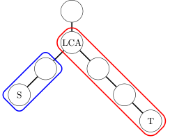
Summing bottom-up amounts to computing prefix sums over these two ranges from the bottom up. Comparing this with the 1D difference update above shows why vertex difference is correct.
Edge difference
To add \(v\) to every edge weight on the path between nodes \(x\) and \(y\), update the difference array \(\{D_x\}\) as follows:
After all updates, computing the subtree sums once yields the updated edge weights (each stored at the child end of its edge).
Example
As the figure shows, edge difference solves range addition on the edge weights along the red path.
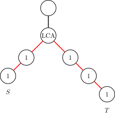
Differencing directly on edges is awkward, so the values that should accumulate on the red edges are moved down into the adjacent nodes, where they are easy to handle. Comparing with the formulas for vertex difference explains the formulas for edge difference.
Example problems
[USACO15DEC] Max Flow
FJ has installed \(N-1\) pipes between the \(N(2 \le N \le 50,000)\) stalls of his barn, which are numbered from \(1\) to \(N\). The pipes connect all the stalls.
FJ has \(K(1 \le K \le 100,000)\) routes for transporting milk; the \(i\)-th route runs from stall \(s_i\) to stall \(t_i\). A route adds one unit of transport pressure to the stalls at its two endpoints and to every stall it passes through on the way. Compute the pressure of the stall under the greatest pressure.
Approach
We need the number of times each node is passed through. Use difference on trees to add one to every node on the path of each route; this quickly gives the count for every node. Here the LCA is computed by binary lifting. Finally, a DFS traverses the whole tree and sums the difference array as it backtracks, which gives the answer.
Reference code
1 2 3 4 5 6 7 8 9 10 11 12 13 14 15 16 17 18 19 20 21 22 23 24 25 26 27 28 29 30 31 32 33 34 35 36 37 38 39 40 41 42 43 44 45 46 47 48 49 50 51 52 53 54 55 56 57 58 59 60 61 62 63 64 65 66 67 68 69 70 71 72 73 74 75 76 77 78 | |
Practice problems
Prefix sums:
- Luogu B3612 [Advanced 1, Example 1] Range Sum
- Luogu U69096 Inverse of Prefix Sums
- AtCoder joi2007ho_a Maximum Sum
- [USACO16JAN] Subsequences Summing to Sevens
- [USACO05JAN] Moo Volume S
2D and multidimensional prefix sums:
- HDU 6514 Monitor
- Luogu P1387 Largest Square
- [HNOI2003] Laser Bomb
- CF 165E Compatible Numbers
- CF 383E Vowels
- ARC 100C Or Plus Max
Prefix sums on trees:
Difference arrays:
2D and multidimensional difference arrays:
Difference on trees:
- [USACO15DEC] Max Flow
- JLOI2014 The Squirrel's New Home
- NOIP2015 Transport Plan
- NOIP2016 Love Running Every Day
This page is an unofficial English translation of the original OI Wiki page (revision 9bb3a8e6), machine-translated by Claude Fable 5.2 on 2026-11-16. It has been modified from the original by translation and may contain errors. It is not endorsed by OI Wiki.
Found a translation problem? Report it on GitHub.
Authors of the original page: Planet6174, zirnc, 24OI-bot, Ir1d, Alpha1022, LeoJacob, sshwy, ouuan, diauweb, Henry-ZHR, H-J-Granger, ShaoChenHeng, Chrogeek, NachtgeistW, leoleoasd, Enter-tainer, Alpacabla, ksyx, Early0v0, Backl1ght, Junyan721113, kenlig, StudyingFather, iamtwz, LeiJinpeng, Tiphereth-A, shawlleyw, c-forrest, Kaiser-Yang, Developer09264, HeRaNO (full contribution history)
All content on this page is provided under the terms of CC BY-SA 4.0 and SATA; additional terms may apply.