Binary Search
This page gives a brief introduction to binary search, binary search on the answer, and ternary search, a technique derived from binary search.
Binary search
Binary search, also known as half-interval search or logarithmic search, is an algorithm for finding an element in a sorted sequence.
Procedure
As an example, consider finding a number in an array sorted in ascending order.
At each step, binary search looks at the middle element of the part of the array still under consideration. If the middle element is the one we want, the search ends. If it is smaller than the target, then every element to its left is no larger than it and cannot be the target, so we only need to search the right side. If it is larger than the target, the same argument shows that we only need to search the left side.
Concretely, let the array \(a\) be indexed from \(1\) and have length \(n\), and suppose we want to find the position of the number \(x\). We maintain \(l\) and \(r\) such that only the elements whose index \(i\) satisfies \(l\le i\le r\) are still under consideration. Initially, set \(l\gets1\) and \(r\gets n\). At each step, look at the middle element \(a_{\textit{mid}}\), where \(\textit{mid}=\left\lfloor\dfrac{l+r}{2}\right\rfloor\), and distinguish three cases:
- If \(a_{\textit{mid}}<x\): the array is ascending, so every element with index at most \(\textit{mid}\) is smaller than \(x\). None of them needs to be examined, and we only have to search the elements with index greater than \(\textit{mid}\). That is, set \(l\gets \textit{mid}+1\) and leave \(r\) unchanged.
- If \(a_{\textit{mid}}>x\): the array is ascending, so every element with index at least \(\textit{mid}\) is larger than \(x\). None of them needs to be examined, and we only have to search the elements with index less than \(\textit{mid}\). That is, leave \(l\) unchanged and set \(r\gets \textit{mid}-1\).
- If \(a_{\textit{mid}}=x\), we have found the position of \(x\) and the algorithm ends.
If the part under consideration becomes empty (\(l>r\)) before the position of \(x\) has been found, then \(x\) is not in the array \(a\).
Properties
Time complexity
The best-case time complexity of binary search is \(O(1)\).
Its average-case time complexity and worst-case time complexity are both \(O(\log n)\). Each step halves the interval left to search, so for an array of length \(n\) the algorithm makes at most \(O(\log n)\) comparisons with the target.
Space complexity
The iterative version of binary search uses \(O(1)\) space.
The recursive version (without tail-call elimination) uses \(O(\log n)\) space.
Implementation
1 2 3 4 5 6 7 8 9 10 11 12 13 14 15 | |
Note
-
For a signed \(s\) that you can guarantee satisfies \(s\ge 0\),
s >> 1compiles to fewer instructions thans / 2; see the section on replacing multiplication with shifts in Compiler Optimizations. -
When \(l\) or \(r\) is very large, \(l+r\) may overflow. If \(r-l\) does not overflow in that situation, replace
(l + r) >> 1in the code withl + ((r - l) >> 1).
Warning
When \(s\) is a negative odd number, s >> 1 and s / 2 are not the same: the results differ by \(1\). The former rounds toward negative infinity (standardized in C++20, implementation-defined before that), while the latter rounds toward zero. See C++ bitwise operators. So when \(l + r\) may be negative, (l + r) / 2 can evaluate to \(r\), and an implementation that updates with r = mid then enters an infinite loop. For example, when \(l = -1,~r = 0\), (l + r) / 2 equals \(0\). Keep this difference in mind when you write the code.
bsearch
bsearch is the binary search provided by the C standard library, declared in <stdlib.h>. In the C++ standard library it is declared in <cstdlib>. qsort and bsearch are the only two algorithmic functions in the C standard library.
Compared with the four parameters of qsort (see Sorting in the STL), bsearch has one more parameter at the far left: the address of the element to search for. It is passed by address so that the comparison function written for qsort can be reused as is, which lets you search immediately after sorting. This means you cannot pass a value directly: store the value in a variable first, then pass the address of that variable.
bsearch therefore takes five parameters: the address of the element to search for, the address of the first array element, the number of elements, the size of an element, and the comparison rule. The comparison rule is again given by a comparison function; see Sorting in the STL.
bsearch returns the address of the element it found; the return type is void *.
Note that bsearch differs in two ways from std::lower_bound and std::upper_bound, which are introduced below:
- When several elements match, it is unspecified which of them is returned.
- When no matching element is found, it returns
NULL.
lower_bound can do almost everything bsearch does (handling the not-found case separately makes the two behave identically), so a solution that passes a problem with bsearch still passes when it is rewritten directly with lower_bound.
Binary search on the answer
Binary search on the answer exploits a generalized ordering property of the answer to a problem (usually called monotonicity) to find the answer quickly, in much the same way as binary search.
Unless stated otherwise, binary search on the answer refers to the integer version, in which the answer is known to be an integer.
Problems that can be solved this way usually have the form "find the largest (or smallest) value that satisfies condition \(P\)" and have the following properties:
- Given any number \(x\), it is easy to decide whether \(x\) satisfies the condition.
- The answer has rough lower and upper bounds: we can find \(L\) and \(R\) such that if an answer \(x\) exists, then \(L\le x \le R\).
- The interval between these rough bounds is so large that enumerating and testing every candidate would exceed the time limit.
- Condition \(P\) has a generalized ordering property.
Suppose there is a function \(f(x)\) with \(f(x)=1\) if and only if \(x\) satisfies condition \(P\), and \(f(x)=0\) otherwise. The generalized ordering property of \(P\) can then be defined in one of the following ways:
-
\(f(i)\le f(j)\) for all \(L\le i<j \le R\), that is, \(f(x)\) is non-decreasing. Written out as a 0/1 sequence for \(i=L,\dots,R\), the values \(f(i)\) look like
00...011...1. In this case binary search on the answer finds the smallest value that satisfies condition \(P\). -
\(f(i)\ge f(j)\) for all \(L \le i<j \le R\), that is, \(f(x)\) is non-increasing. The corresponding 0/1 sequence looks like
11...100...0. In this case binary search on the answer finds the largest value that satisfies condition \(P\).
In other words, the first ordering property says: if \(x\) satisfies condition \(P\), then so does every number greater than \(x\). Binary search on the answer finds the \(x\) for which every smaller number fails condition \(P\), while \(x\) itself and every larger number satisfy it.
The second ordering property says: if \(x\) satisfies condition \(P\), then so does every number smaller than \(x\). Binary search on the answer finds the \(x\) for which \(x\) itself and every smaller number satisfy condition \(P\), while every larger number fails it.
Procedure
We describe the search for the smallest value (so the problem must have the first ordering property above). Let the rough bounds on the answer be \(L\) and \(R\).
We maintain \(l\) and \(r\) such that the answer \(x\) is known to satisfy \(l \le x \le r\). As in binary search, initially set \(l\gets L\) and \(r\gets R\). At each step we test whether \(\textit{mid}=\left\lfloor\dfrac{l+r}{2}\right\rfloor\) satisfies condition \(P\) and distinguish two cases:
- If \(\textit{mid}\) does not satisfy the condition (that is, \(f(\textit{mid})\) is \(0\)), then by the ordering property no number less than or equal to \(\textit{mid}\) satisfies it, and none of them needs to be considered. Set \(l\gets \textit{mid}+1\) and leave \(r\) unchanged.
- If \(\textit{mid}\) satisfies the condition (that is, \(f(\textit{mid})\) is \(1\)), then by the ordering property every number greater than or equal to \(\textit{mid}\) satisfies it. But the problem asks for the smallest value, so the numbers greater than \(\textit{mid}\) are of no interest, and only the numbers less than or equal to \(\textit{mid}\) remain. Set \(r \gets \textit{mid}\) and leave \(l\) unchanged.
The algorithm ends when the interval for the answer has shrunk to \(l=r\) (that is, when \(l<r\) no longer holds). At that point \(l\), or equally \(r\), is the answer.
One caveat: if no answer exists within the bounds (what is usually called "no solution"), every query \(f(\textit{mid})\) returns \(0\), so the algorithm ends with \(l=r=R\) and \(f(l)=0\). To detect this case, additionally check whether \(f(l)\) equals \(0\).
As in binary search, each step halves the interval left to search, so the algorithm runs in \(O(M \log (R-L+1))\), where \(M\) is the time needed to test whether \(\textit{mid}\) satisfies condition \(P\).
Implementation
The description above leads to the following implementation:
1 2 3 4 5 6 7 8 9 10 11 12 13 14 15 16 17 18 | |
When -1 stands for "no solution", make sure it cannot be confused with a valid answer.
Implementation details
When reading other people's solutions, you may come across a different implementation:
1 2 3 4 5 6 7 8 9 10 11 12 13 14 15 16 17 | |
The two versions compute the same answer but maintain different loop invariants.
Why do both versions find the smallest feasible value?
First assume that \([L,R]\) is non-empty and contains an answer, and let \(\textit{ans}\) be the smallest number that satisfies condition \(P\). Since \(f\) is non-decreasing, on the original interval \([L,R]\) we have
The l < r version keeps the answer inside a closed interval.
The invariant it maintains is
Each iteration takes \(\textit{mid}=\left\lfloor\dfrac{l+r}{2}\right\rfloor\). If \(f(\textit{mid})=1\), then \(\textit{ans}\le\textit{mid}\), and we set \(r\gets\textit{mid}\); if \(f(\textit{mid})=0\), then \(\textit{ans}>\textit{mid}\), and we set \(l\gets\textit{mid}+1\). Both updates preserve the invariant.
When \(l<r\), we have \(l\le\textit{mid}<r\), so every iteration strictly shrinks the interval. The loop ends with \(l=r\), and the invariant gives \(\textit{ans}=l\).
The l <= r version discards the part that is already decided, and the answer may sit one position past the right boundary.
The invariant it maintains is: within the original interval \([L,R]\), every \(x<l\) satisfies \(f(x)=0\) and every \(x>r\) satisfies \(f(x)=1\). Given that an answer exists, this means
If \(f(\textit{mid})=1\), then every \(x\ge\textit{mid}\) in the original interval satisfies \(f(x)=1\), so we may set \(r\gets\textit{mid}-1\); if \(f(\textit{mid})=0\), then every \(x\le\textit{mid}\) in the original interval satisfies \(f(x)=0\), so we may set \(l\gets\textit{mid}+1\).
Every iteration removes at least one integer from the interval still to be searched, so the loop eventually ends.
While the loop runs, \(l\le\textit{mid}\le r\). After \(r\gets\textit{mid}-1\), the new right boundary satisfies \(r\ge l-1\); after \(l\gets\textit{mid}+1\), the new left boundary satisfies \(l\le r+1\). Whichever update is applied, \(l\le r+1\) holds afterwards. The loop ends when \(l>r\), and since the boundaries are integers this forces \(l=r+1\). Together with the invariant \(l\le\textit{ans}\le r+1\) on the position of the answer, this gives \(\textit{ans}=l\).
Note that the interval \([l,r]\) still to be searched does not always contain the answer. For example, if an iteration happens to pick \(\textit{mid}=\textit{ans}\), then after \(r\gets\textit{mid}-1\) we have \(\textit{ans}=r+1\). The answer is no longer in \([l,r]\), but it still satisfies the invariant \(l\le\textit{ans}\le r+1\), so the correctness proof above is unaffected.
When there is no solution, the two versions stop at different positions.
For the l <= r version: if \(l\le R\) when the loop ends, then \(l\) lies in the original interval, because the left boundary always satisfies \(l\ge L\). From \(l=r+1\) and the invariant that every \(x>r\) in the original interval satisfies \(f(x)=1\), it follows that \(f(l)=1\), so there is no need to call check(l) again.
If there is no solution, the loop ends with \(l=R+1\), which is outside the original search interval. We only require check to be usable on \([L,R]\), so test l > R first; do not call check(l) directly to decide whether a solution exists.
For the l < r version, recall from the description earlier that if the interval contains no solution, the loop ends with \(l=r=R\). An extra test of whether check(l) is \(0\) is then needed to tell an answer of \(R\) apart from no solution.
In summary, provided that \(L\le R\) and \(f\) is non-decreasing on \([L,R]\), both versions end after finitely many iterations. If the interval contains a feasible value, both end with \(l=\textit{ans}\) and return the smallest integer in the interval that satisfies the condition. If it contains no solution, the l < r version detects this with check(l) after the loop and the l <= r version with l > R, and both return the agreed no-solution marker. For an empty interval with \(L>R\), both pieces of code return the no-solution marker before entering the loop. So although the two implementations maintain different loop invariants and stop at different positions, both correctly answer the query for the smallest feasible value and return the same result.
These two versions show that the correctness of a binary search implementation depends on how the meaning of the boundaries, the loop invariant, the loop condition and the update rules fit together. Whether the interval endpoints are included, or whether the loop uses l < r or l <= r, is not enough to tell whether an implementation is correct.
To prove an implementation correct, check the following:
- Initialization establishes the loop invariant.
- Every update preserves the invariant and strictly decreases the number of integers in the interval still to be searched, which guarantees that the loop eventually ends.
- When the loop ends, the invariant and the termination condition together determine that the returned value is the answer. If there may be no solution, you also have to explain how that case is recognized.
When discussing implementations, take care to distinguish the interval that is still to be searched from the interval that is guaranteed to contain the final answer. Depending on the boundary conditions the two need not coincide, and we cannot require of every variant that the answer always lie in the interval still to be searched.
The table below lists several common variants. All of them assume \(L\le R\), that the problem has the first ordering property, and that the smallest feasible value \(\textit{ans}\) exists. For the position of the answer, the column "Invariant on the answer" is authoritative.
| Variant | Initial \(l,r\) | Loop condition | \(\textit{mid}\) | When \(f(\textit{mid})=1\) | When \(f(\textit{mid})=0\) | Invariant on the answer | At exit | Return |
|---|---|---|---|---|---|---|---|---|
| Closed interval \([l,r]\), discarding the decided part | \(l=L,\ r=R\) | \(l\le r\) | \(\left\lfloor\dfrac{l+r}{2}\right\rfloor\) | \(r\gets\textit{mid}-1\) | \(l\gets\textit{mid}+1\) | \(l\le\textit{ans}\le r+1\) | \(l=r+1\) | \(l\) |
| Closed interval \([l,r]\), keeping the answer | \(l=L,\ r=R\) | \(l<r\) | \(\left\lfloor\dfrac{l+r}{2}\right\rfloor\) | \(r\gets\textit{mid}\) | \(l\gets\textit{mid}+1\) | \(l\le\textit{ans}\le r\) | \(l=r\) | \(l\) |
| Half-open interval \([l,r)\), discarding the decided part | \(l=L,\ r=R+1\) | \(l<r\) | \(\left\lfloor\dfrac{l+r}{2}\right\rfloor\) | \(r\gets\textit{mid}\) | \(l\gets\textit{mid}+1\) | \(l\le\textit{ans}\le r\) | \(l=r\) | \(l\) |
| Interval \((l,r]\), open on the left and closed on the right, keeping the answer | \(l=L-1,\ r=R\) | \(l+1<r\) | \(\left\lfloor\dfrac{l+r}{2}\right\rfloor\) | \(r\gets\textit{mid}\) | \(l\gets\textit{mid}\) | \(l<\textit{ans}\le r\) | \(l+1=r\) | \(r\) |
| Open interval \((l,r)\), maintaining a boundary on each side | \(l=L-1,\ r=R+1\) | \(l+1<r\) | \(\left\lfloor\dfrac{l+r}{2}\right\rfloor\) | \(r\gets\textit{mid}\) | \(l\gets\textit{mid}\) | \(l<\textit{ans}\le r\) | \(l+1=r\) | \(r\) |
A few remarks on the table:
- In row 3, \([l, r)\) is the interval still to be searched, but the answer may be exactly \(r\).
- Row 4 keeps the answer inside \((l, r]\), which relies on the initial right boundary \(R\) satisfying \(f(R) = 1\). While the loop runs, \(r - l \ge 2\), so rows 4 and 5 stay correct if the midpoint is computed with the ceiling instead.
- In row 5, \((l, r)\) denotes the positions between the two boundaries that are still undecided. Think of the initial \(L - 1\) as a virtual sentinel with value 0 and of \(R + 1\) as a virtual sentinel with value 1. The loop calls the check function only inside the original interval, so the function never actually has to be evaluated at the sentinels.
- To handle the no-solution case: in rows 1, 3 and 5, test whether the returned value is \(R + 1\); in row 2, check \(f(l)\); in row 4, check \(f(R)\) beforehand.
Minimizing the maximum and maximizing the minimum
Minimizing a maximum and maximizing a minimum are typical problems that binary search on the answer can solve.
Take minimizing the maximum. Usually each configuration corresponds to a set \(S\) that has to be considered. If the task is to minimize, over all configurations, the maximum of the numbers in the corresponding set \(S\), we can restate it as: find the smallest \(k\) for which some configuration satisfies \(\max(S) \le k\).
This problem has the generalized ordering property: if a configuration satisfies \(\max(S) \le k\), then for \(i\ge k\) it also satisfies \(\max(S)\le i\). So for every \(i \ge k\) there is a configuration with \(\max(S) \le i\), and \(i\) meets the condition of the problem as well. Binary search on the answer therefore applies. Maximizing the minimum works the same way.
Binary search on the answer in the STL
std::lower_bound and std::upper_bound
The C++ standard library provides:
std::lower_bound, which finds the first element not less than a given value.std::upper_bound, which finds the first element greater than a given value.
Both are implemented with binary search, so the elements must be ordered before the call (ordered with respect to the comparison function described below, which need not be an order in the mathematical sense). Only then do the two problems have the generalized ordering property: for std::lower_bound, if \(a_i\) is not less than the given value, neither is any element after position \(i\); for std::upper_bound, if \(a_i\) is greater than the given value, so is every element after position \(i\).
std::lower_bound and std::upper_bound each take four parameters:
first: the begin iterator of the sequence, which points to its first element.last: the end iterator of the sequence, which points to the position one past its last element. In other words, iflastis a bidirectional iterator,--lastpoints to the last element of the sequence.value: the given value.comp(optional): the comparison function, written the same way as forsort. Note thatstd::lower_boundcalls it ascomp(element, value), whereasstd::upper_boundcalls it ascomp(value, element).
Both return an iterator to the element that satisfies the condition, of the same type as the iterators passed in. That is, if you pass array pointers, you get back a pointer to the array element that satisfies the condition. If no element satisfies it, last is returned.
Both are defined in the header <algorithm>.
Usage examples
- In an array \(a\) of length \(n\) indexed from \(1\), find the first number not less than \(x\) among positions \(l\) to \(r\) and get its index:
lower_bound(a+l,a+r+1,x)-a. - In an array \(a\) of length \(n\) indexed from \(0\), find the first number greater than \(x\) (such a number must exist) and get its value:
*upper_bound(a,a+n,x). - In a vector \(a\) of length \(n\), find the first number not less than \(x\) and get its index (vector indices start at \(0\)):
lower_bound(a.begin(),a.end(),x)-a.begin().
About iterators
The begin and end iterators above must be ForwardIterators. Array pointers and the iterators of vector, set, map and string all meet this requirement.
About the time complexity
In libstdc++, the standard library implementation used by GCC, both functions use std::advance to reach the middle element. So they run in \(O(\log n)\) only when the iterators support random access (when you pass array pointers or vector iterators, for example). Without random access (set or map, for example), the cost is the sum of the costs of reaching each middle element, which is usually linear. For example, a call like lower_bound(st.begin(),st.end(),val) on a set or map takes \(O(n)\) time. Use the member function st.lower_bound(val) instead.
Implementing std::lower_bound and std::upper_bound with bsearch
bsearch returns NULL when it cannot find the element (see bsearch), for example when searching for 3 in the sequence 1, 2, 4, 5, 6. This makes it hard to get the behavior of lower_bound out of bsearch.
To implement std::lower_bound and std::upper_bound with bsearch, use the convention on the arguments of its comparison function: the first argument points to the element being searched for, the second to an element of the array being searched. So it suffices for the comparison function to know the address of the first array element.
1 2 3 4 5 6 7 8 9 10 11 12 13 14 15 16 17 18 19 20 21 22 23 24 25 26 27 28 29 | |
Note that if the answer is the past-the-end position (for example, when the element searched for is greater than every element), this method still returns NULL, and that case has to be handled separately.
OI contestants today rarely write pure C, and this technique is of limited use, so it is not important. Beginners should simply use the C++ functions std::lower_bound and std::upper_bound.
std::partition_point
C++11 introduced std::partition_point. Given a partitioned sequence, it uses binary search on the answer to locate the partition point quickly.
std::partition_point takes three parameters:
first,last: as above.p: a unary predicate. This is a callable object that accepts one argument \(v\) and returns a Boolean value telling whether \(v\) satisfies the partition condition.
Let \(a\) be the sequence passed in. The function returns an iterator to the first element that does not satisfy the partition condition, that is, an iterator to the element with the smallest index \(x\) for which \(p(a_x)\) equals false.
The sequence must be partitioned, that is, it must have the second generalized ordering property described above. In other words, if we write the results \(p(v)\) for the elements \(v\) of the sequence as a 0/1 sequence, it looks like 11...100...0, and the function returns an iterator to the position of the first \(0\).
How std::partition_point relates to std::lower_bound and std::upper_bound
In fact, std::lower_bound and std::upper_bound are special cases of std::partition_point.
Define a function f with the code bool f(int v) { return !(val <= v); }. Passing f to std::partition_point as the predicate gives the same result as std::lower_bound. std::upper_bound is analogous.
Binary search on a real-valued answer
Binary search on a real-valued answer, also called floating-point binary search, is the form binary search on the answer takes when the answer is a real number.
Unlike the integer version, it usually does not have to produce the exact answer, only a real approximation that meets a given precision requirement.
Procedure
We describe the search for the smallest value. Let the rough bounds on the answer be \(L\) and \(R\), and maintain \(l\) and \(r\) such that the answer \(x\) is known to satisfy \(l\le x\le r\). Initially, set \(l\gets L\) and \(r\gets R\). At each step take \(\textit{mid}=\dfrac{l+r}{2}\) (note that this is real arithmetic) and test whether \(\textit{mid}\) satisfies condition \(P\):
- If \(\textit{mid}\) satisfies the condition, then much as in the integer case, set \(r\gets \textit{mid}\) and leave \(l\) unchanged.
- If \(\textit{mid}\) does not satisfy the condition, then much as in the integer case, set \(l\gets \textit{mid}\) and leave \(r\) unchanged.
Unlike the integer version, the real-valued version cannot shrink the interval with mid + 1 or mid - 1, because the real numbers have no adjacent elements. All it can do is move a boundary to \(\textit{mid}\) and rely on the repeated halving of the interval length to close in on the answer.
The algorithm ends when the interval length \(r-l\) is at most the given precision \(\textit{eps}\), or when a preset number of iterations has been reached. At that point \(l\), \(r\) or \(\dfrac{l+r}{2}\) can each serve as an approximation of the answer (return \(r\) if the returned value itself must satisfy condition \(P\)). To find the largest value, just reverse the direction of the two cases: if \(\textit{mid}\) satisfies the condition, set \(l\gets \textit{mid}\); otherwise set \(r\gets \textit{mid}\) (and correspondingly, return \(l\) if the returned value itself must satisfy condition \(P\)).
With while (r - l > eps), binary search on a real-valued answer runs in \(O(M \log((R-L)/\textit{eps}))\). With a fixed number of iterations \(k\), it runs in \(O(Mk)\). Here \(M\) is the time needed to test whether \(\textit{mid}\) satisfies condition \(P\). Because real arithmetic is subject to floating-point error, implementations usually do not test \(l=r\) directly. They test \(r-l<\textit{eps}\) instead, or simply loop a fixed number of times, for example \(60\) to \(100\), which avoids an infinite loop and guarantees the precision.
Implementation
1 2 3 4 5 6 7 8 9 10 11 12 13 14 15 16 17 18 19 20 21 22 23 24 25 | |
Warning
Do not make eps too large, or the result will not be precise enough. Do not make it too small either, or floating-point error may keep the loop from ever reaching it, and the loop runs forever. If the answer range is very large or the required precision is very high, use a fixed number of iterations rather than while (r - l > eps).
Example problems
Luogu P1873 Cutting Trees
Mirko the lumberjack needs to cut down \(M\) meters of wood. This is an easy job for him, because he has a shiny new wood-cutting machine that goes through a forest like wildfire. However, Mirko is only allowed to cut a single row of trees.
The machine works as follows. Mirko sets a height parameter \(H\) (in meters), the machine raises a giant saw blade to height \(H\) and cuts off every part of a tree that is above \(H\) (the parts of the trees that are not above \(H\) meters stay as they are, of course). Mirko then gets the parts that were cut off.
For example, if the trees in a row have heights \(20,~15,~10,~17\) and Mirko raises the blade to a height of \(15\) meters, the remaining heights after cutting are \(15,~15,~10,~15\), and Mirko gets \(5\) meters of wood from the first tree and \(2\) meters from the fourth, \(7\) meters in total.
Mirko cares a great deal about protecting the environment, so he will not cut off more wood than he has to. That is why he sets the saw blade as high as he can. Your task is to help Mirko find the largest integer height \(H\) of the saw blade for which he still gets at least \(M\) meters of wood. In other words, if the blade were raised by \(1\) more meter, he would no longer get \(M\) meters of wood.
Approach
We could enumerate the answers from \(0\) to \(10^9\), but this naive approach will certainly not get full marks, because going all the way from \(0\) to \(10^9\) takes too long. Instead, we binary search for the answer on the interval \([0,~10^9]\) and check the feasibility of each candidate answer (usually with a greedy method). This is binary search on the answer.
Reference code
1 2 3 4 5 6 7 8 9 10 11 12 13 14 15 16 17 18 19 20 21 22 23 24 25 26 27 28 29 30 31 32 33 | |
After reading the code above, you will surely have two questions:
-
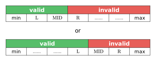
Why is the search interval half-open?
Because at the end of the search we arrive at this (shown for the largest valid value):
and then at this:
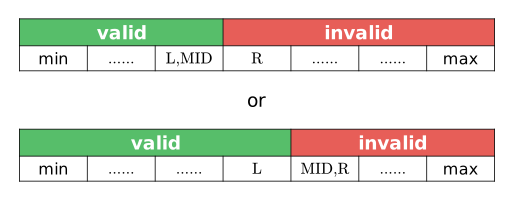
For the smallest valid value it is exactly the other way around.
-
Why is the left value returned?
For the same reason. When the loop ends, \(l+1=r\),
check(l)is true andcheck(r)is false, so \(l\) is the largest valid value.
Ternary search
Introduction
The bisection method can approximate a zero of a function. To find the extremum point of a unimodal function, the usual tool is ternary search.
This section uses the following strict convention for unimodality: a function \(f(x)\) defined on \([l,r]\) is called a unimodal function if there is an \(x^*\in[l,r]\) such that \(f(x)\) is strictly increasing on \([l,x^*]\) and strictly decreasing on \([x^*,r]\). Both intervals include \(x^*\), so \(x^*\) is the unique maximizer and \(f(x^*)\) is the maximum.
Why not find the extremum point as a zero of the derivative?
First, unimodality does not guarantee that the derivative has a unique zero, and a point where the derivative is zero need not be the maximizer. For example, take
The zeros of \(f'(x)\) are \(x=1\) and \(x=3\), whereas \(f(x)\) attains its maximum at \(x=2\), where it is not differentiable.
Second, for some functions both the differentiation and its result are complicated, and some functions cannot even be written in the form \(y=f(x)\).
Finally, in some problems the unimodal function whose extremum point we need is not a single function but the result of combining several functions by a special operation (for example, when maximizing the minimum of several linear functions that are not all monotone in the same direction). Its derivative may then be a piecewise function, and the function may fail to be differentiable at some points.
Note
Ternary search can find the maximum of a unimodal function and, equally, the minimum of a function with a single valley. For convenience, the rest of this page always takes finding the maximum of a unimodal function as the example, unless stated otherwise.
Procedure
The basic idea of ternary search is similar to that of binary search, but each step picks two arbitrary points \(\textit{lmid} < \textit{rmid}\) (the two blue points in the figure below) in the current interval \([l,r]\) (between the two orange points in the figure). As the figure shows, if \(f(\textit{lmid})<f(\textit{rmid})\), the function must be increasing on \([l,\textit{lmid})\) (the red part of the figure), so the maximizer (the green point) cannot lie in that interval and the interval can be discarded. However, we cannot rule out that the maximizer lies to the right of \(\textit{rmid}\), so nothing more can be discarded. The opposite case is symmetric.
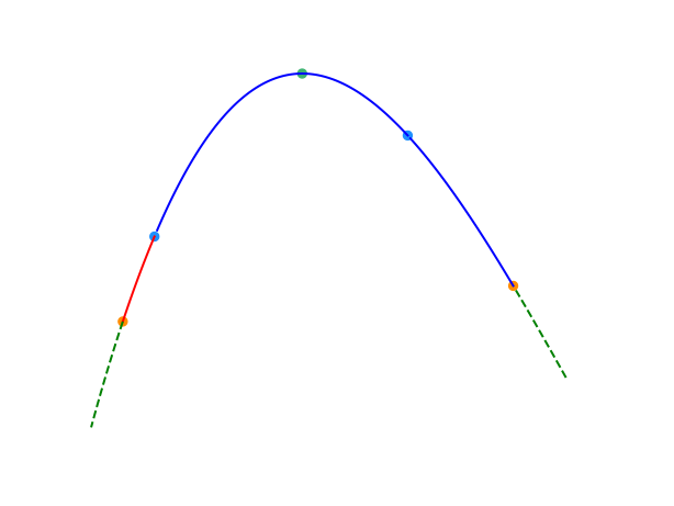
The correctness of ternary search does not depend on the particular choice of \(\textit{lmid}\) and \(\textit{rmid}\): they only have to be two distinct points in the interval, and the two points that divide it into thirds are a common choice. The choice does affect the efficiency of ternary search, though. Each step discards one of the two outer intervals, so we can also take two split points close to the midpoint to make the discarded interval larger. If we take \(\textit{mid}\pm\delta\) with \(\delta>0\) small enough, comparing the two function values amounts to determining the sign of the approximate derivative \(\dfrac{f(\textit{mid}+\delta)-f(\textit{mid}-\delta)}{2\delta}\). The functions met in competitive programming are usually nicely smooth, so this tells us roughly on which side of \(\textit{mid}\) the extremum point lies, and the efficiency comes close to that of the bisection method.
Implementation
The pseudocode is as follows:
Choosing the split points
The code above takes \(\textit{mid} \pm \varepsilon / 3\) as the split points so that they always lie between the current \(l\) and \(r\), which keeps the algorithm out of an infinite loop.
The integer case
If the domain of \(f(x)\) is the integers, both the ternary search above and the golden-section search described below should stop as soon as \(r-l\) is small. When \(r-l\) is small, find the maximizer by brute force, going through all the remaining points.
Optimization: golden-section search
If a single call to \(f(x)\) is expensive and the number of calls has to be reduced further, golden-section search improves the constant factor of ternary search. It is also an important part of the optimum seeking method put forward by Hua Luogeng.
In ternary search, each iteration needs two function calls, and one iteration shrinks the interval to \(1/2\) of its previous length at best. So reaching precision \(\varepsilon\) takes at least
function calls. This is the best that ternary search can achieve. With other split points, such as the points that divide the interval into thirds, the number of calls grows further, because one iteration shrinks the interval more slowly.
Golden-section search improves on this by reusing split points that have already been evaluated. Apart from the first iteration, which needs two function calls, every iteration then needs only one. Let the golden ratio be
In each iteration, the split points are the left and right golden-section points:
Golden-section points divide a line segment in a self-similar way: \(m^l\) is the left golden-section point of the segment \([l,r]\) and also the right golden-section point of the segment \([l,m^r]\). The benefit of choosing the split points this way is that in every iteration \(k>1\), one of the two split points has already been evaluated, so the earlier result can be reused directly.
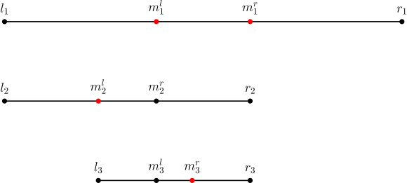
With the split points chosen this way, reaching precision \(\varepsilon\) takes only
function calls. Asymptotically, the function is called fewer times.
The pseudocode is as follows:
Example problems
Luogu P3382 - Ternary Search
Given a polynomial function of degree \(N\) and a range \([l, r]\), find the unique value of \(x\) such that the function is increasing on \([l, x]\) and decreasing on \([x, r]\).
Approach
The problem asks for the argument at which a polynomial function of degree \(N\) attains its maximum on \([l, r]\), so ternary search clearly applies. The implementation below uses the two points that divide the interval into thirds and moves an endpoint of the interval to the split point that was actually compared. Once the interval is short enough, it prints the midpoint of the interval.
Reference code
1 2 3 4 5 6 7 8 9 10 11 12 13 14 15 16 17 18 19 20 21 22 23 24 25 26 27 28 29 30 | |
1 2 3 4 5 6 7 8 9 10 11 12 13 14 15 16 17 | |
Practice problems
- UVa 1476 - Error Curves
- UVa 10385 - Duathlon
- UOJ 162 - [Tsinghua training camp 2015] Light Bulb Testing
- Luogu P7579 - [RdOI R2] Weighing (weigh)
Fractional programming
See also: Fractional Programming
Fractional programming is usually stated as the following problem: each item has two attributes \(c_i\) and \(d_i\), and we must select some of the items in some way so that \(\dfrac{\sum{c_i}}{\sum{d_i}}\) is as large or as small as possible.
Classic examples include the optimal ratio cycle and the optimal ratio spanning tree.
Fractional programming can be solved with binary search.
References and notes
This page is an unofficial English translation of the original OI Wiki page (revision 9bb3a8e6), machine-translated by Claude Fable 5.2 on 2026-11-16. It has been modified from the original by translation and may contain errors. It is not endorsed by OI Wiki.
Found a translation problem? Report it on GitHub.
Authors of the original page: Ir1d, HeRaNO, Xeonacid, i-yyi, 24OI-bot, billchenchina, cbw2007, zirnc, Marcythm, flylai, sshwy, HanwGeek, StudyingFather, Henry-ZHR, H-J-Granger, Konano, Enter-tainer, NachtgeistW, leoleoasd, ksyx, Great-designer, Selflocking, yusancky, shuzhouliu, iamtwz, inclyc, LeiJinpeng, Tiphereth-A, shawlleyw, w-tianshui, gavinliu266, FinParker, c-forrest, TH911, TOMWT-qwq, hhc0001, Tokur233, liangbob2023, not-exist (full contribution history)
All content on this page is provided under the terms of CC BY-SA 4.0 and SATA; additional terms may apply.