Sparse Table
Definition
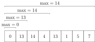
A sparse table (ST) is a data structure for solving idempotent range query problems.
What is an idempotent range query problem?
A range query problem is idempotent if its operation \(\operatorname{opt}\) satisfies \(x\operatorname{opt} x=x\). For example, \(\max(x,x)=x\) and \(\operatorname{gcd}(x,x)=x\), so RMQ and range GCD are idempotent range query problems. Range sum is not: if the precomputed ranges used to answer a query overlap, the overlap is counted twice, which is not what we want. A sparse table also requires \(\operatorname{opt}\) to be associative.
What is RMQ?
RMQ stands for Range Maximum/Minimum Query: finding the maximum (or minimum) over a range. There are many ways to solve it; see the RMQ topic page.
Introduction
Luogu P3865 [Template] Sparse Table & RMQ Problem
You are given \(n\) (\(1\le n\le 10^5\)) integers and \(m\) (\(1\le m\le 2\times 10^6\)) queries. For each query, find the maximum over the range \([l,r]\).
Consider brute force first: for each query, scan the range \([l,r]\) and take the maximum.
Clearly, this is too slow to pass the time limit.
Sparse table
A sparse table is built on binary lifting. After \(\Theta(n\log n)\) preprocessing it answers each query in \(\Theta(1)\), but it does not support updates.
How can binary lifting give us a range maximum? If we apply it in the usual way, jumping \(2^i\) steps at a time, a query still takes \(\Theta(\log n)\). That is no faster than a segment tree, and the preprocessing is slower.
But \(\max(x,x)=x\): the range maximum is idempotent. So the precomputed ranges we combine are allowed to overlap, and the answer is still correct as long as their union is exactly the queried range.
Trying a few cases by hand shows that two precomputed ranges are always enough to cover a queried range. A query therefore takes only \(\Theta(1)\), which makes a real difference when there are many queries.
Here are the details.
Let \(f(i,j)\) denote the maximum over the range \([i,i+2^j-1]\).
Clearly \(f(i,0)=a_i\).
In binary lifting terms, the second index means "jump \(2^j-1\) steps", which gives the recurrence \(f(i,j)=\max(f(i,j-1),f(i+2^{j-1},j-1))\).
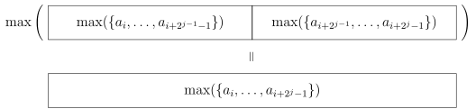
That is all there is to the preprocessing. Queries are just as simple.
We cover each query \([l,r]\) with two ranges, \([l,l+2^s-1]\) and \([r-2^s+1,r]\), where \(s=\left\lfloor\log_2(r-l+1)\right\rfloor\). The answer is the larger of their two maxima.
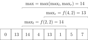
As argued above, the maximum is idempotent, so the overlap between the two ranges does no harm. And since together they cover exactly \([l,r]\), the answer is correct.
Luogu P3865 [Template] Sparse Table & RMQ Problem reference implementation
1 2 3 4 5 6 7 8 9 10 11 12 13 14 15 16 17 18 19 20 21 22 23 24 25 26 27 28 29 30 31 32 | |
1 2 3 4 5 6 7 8 9 10 11 12 13 14 15 16 17 18 19 20 21 22 23 24 25 26 27 28 29 30 31 32 33 34 35 36 37 38 39 40 41 42 43 44 45 46 47 48 49 50 51 52 53 54 55 56 57 58 59 60 | |
1 2 3 4 5 6 7 8 9 10 11 12 13 14 15 16 17 18 19 20 21 22 23 24 25 26 27 28 29 30 31 32 33 34 35 36 37 | |
Caveats
-
The input and output are usually large, so use fast I/O.
-
The table is usually a two-dimensional array, with \(\log n\) entries along one dimension and \(n\) along the other. Put the \(\log n\) dimension first: this improves cache locality.
-
Calling std::log on every query is wasteful. Use a built-in such as
__builtin_clzor__lginstead; if none is available, precompute the logarithms like this:
Sparse tables for other operations
RMQ is not the only idempotent range query problem. Range bitwise AND, range bitwise OR and range GCD are others, and a sparse table handles all of them efficiently.
For range GCD, though, a sparse table query is asymptotically no faster than a segment tree query. (If the values are at most \(w\), a sparse table query takes \(\Theta(\log w)\) and a segment tree query \(\Theta(\log n+\log w)\), and the bound on the values is usually larger than \(n\).) On the other hand, its preprocessing is no slower than a segment tree's, and it is much simpler to code.
Looked at closely, idempotent range query problems tend to have an RMQ hidden inside them. Range bitwise AND is a minimum taken bit by bit, and range GCD is a minimum taken over the exponent of each prime factor.
Summary
A sparse table is a good fit for idempotent range queries (the operation must also be associative): it is fast and takes far less code than the alternatives. But it works for only a narrow class of operations, is hard to extend, and does not support updates.
Practice problems
Appendix: time complexity of range GCD with a sparse table
Preprocessing takes \(\Theta(\log n)\) iterations, and each of them calls the recursive GCD function. If the values are at most \(w\), one GCD call costs up to \(O(\log w)\), so at first sight the total is \(O(n\log n\log w)\).
However, every recursive step of GCD except the last at least halves some number in the sequence, and the numbers in the sequence can be halved at most \(\log_2 (w^n)=\Theta(n\log w)\) times in total. So the recursive steps number at most \(O(n\log w)\) overall. Adding the \(\Theta(n\log n)\) for the loops (and the last step of each recursion) gives \(O(n(\log w+\log n))\). Inputs can be constructed that force \(\Omega(n(\log w+\log n))\), so the bound is tight: \(\Theta(n(\log w+\log n))\).
Queries are easy to analyze: in the worst case every query hits the worst possible pair of numbers and costs \(\Theta(\log w)\). So range GCD on a sparse table takes \(\Theta(n(\log n+\log w))\) to preprocess and \(\Theta(\log w)\) per query.
A segment tree takes \(\Theta(n\log w)\) to preprocess and \(\Theta(\log n+\log w)\) per query.
This argument is not rigorous. A more careful one follows.
A more rigorous proof
This part assumes you know the potential method; see time complexity.
We start with the preprocessing.
Call the sequence at the current level of the preprocessing loop the current sequence, and denote it by \(A\). At level zero it is the original sequence; at level one it is what one iteration makes of that, namely st[1..n][1]; and so on.
Define the potential as the base-two logarithm of the product of all numbers in the current sequence: \(\Phi(A)=\log_2\left(\prod\limits_{i=1}^n A_i\right)\).
The time for one iteration is the time for the loop itself plus the time spent inside GCD. The latter varies: a call may recurse only once or twice, or as many as \(O(\log w)\) times. But every recursive step other than the first and the last at least halves some entry of the current sequence. Each such step lowers \(\Phi(A)\) by at least \(1\), so its cost is amortized against the potential.
Initially \(\Phi(A)\) is at most \(\log_2 (w^n)=\Theta(n\log w)\), and \(\Phi(A)\) never increases. Hence preprocessing the sparse table takes \(O(n(\log w+\log n))\).
This page is an unofficial English translation of the original OI Wiki page (revision 9bb3a8e6), machine-translated by Claude Fable 5.2 on 2026-11-16. It has been modified from the original by translation and may contain errors. It is not endorsed by OI Wiki.
Found a translation problem? Report it on GitHub.
Authors of the original page: Ir1d, ShadowsEpic, 24OI-bot, hsfzLZH1, Xeonacid, Fomalhauthmj, abc1763613206, ouuan, orzAtalod, Henry-ZHR, H-J-Granger, Chrogeek, leoleoasd, Enter-tainer, Great-designer, Backl1ght, kenlig, ksyx, StudyingFather, mcendu, DawnMagnet, shuzhouliu, iamtwz, CCXXXI, Tiphereth-A, zymooll, lbdoknow, purinliang, firogh, hsn8086, c-forrest, HeRaNO (full contribution history)
All content on this page is provided under the terms of CC BY-SA 4.0 and SATA; additional terms may apply.