Integer Factorization
Introduction
Given a positive integer \(N \in \mathbf{N}_{+}\), find one of its nontrivial factors quickly.
Start with the naive algorithm. Divisors come in pairs, so the divisors of \(N\) fall into two blocks, \([2, \sqrt N]\) and \([\sqrt N+1,N)\). It is enough to iterate over the numbers in \([2, \sqrt N]\); division then yields at least two divisors. This method runs in \(O(\sqrt N)\).
For \(N\ge10^{18}\) this running time is unacceptable, and we want a better algorithm. One idea is to guess at random whether a number is a divisor of \(N\). With luck this finds the answer in \(O(1)\) time, but for \(N\ge10^{18}\) a guess succeeds with probability \(\frac{1}{10^{18}}\), and the expected number of guesses is \(10^{18}\). Guessing within \([2,\sqrt N]\) raises the success rate somewhat. We want a way to make the guessing smarter.
Naive algorithm
The simplest algorithm iterates over \([2, \sqrt N]\).
1 2 3 4 5 6 7 8 9 10 11 12 13 | |
1 2 3 4 5 6 7 8 9 10 | |
We can prove that the elements of result are exactly the prime factors of N.
Proof that the elements of result are exactly the prime factors of \(N\)
First look at how N changes. When the iteration for i ends, the part while(N % i == 0) N /= i has just finished, so i no longer divides N. Moreover, every time a factor is divided out, N still divides \(N\). Together these two facts guarantee that when the iteration for i begins, N is a divisor of \(N\) and is not divisible by any integer smaller than i.
Next we show that every element of result is a divisor of \(N\). In the iteration for i, the condition for storing i in result is N % i == 0, which says that i divides N; we have already shown that N is a divisor of \(N\), so i is a divisor of \(N\). When the loop over i ends, N is stored in result as well if it is not one. By the above, it too must be a divisor of \(N\).
Next we show that every element of result is prime. Suppose result contains a composite number \(K\). Then there is an i greater than one and at most \(\sqrt K\) that is a divisor of \(K\). Such a \(K\) cannot have been stored in result as some i of the loop, because the first paragraph showed that when the loop reaches \(K\), N is not divisible by any i smaller than \(K\). Nor can such a \(K\) have been added after the loop: the loop exits when i * i > N, so every i up to \(\sqrt K\) has been visited, and by the above none of these i can divide the current N, which is \(K\).
Finally we show that every prime factor of \(N\) appears in result. Suppose \(p\) is a prime factor of \(N\) that does not appear in result. By the discussion above, \(p\) cannot be an i that occurred in the loop. Let i be the last i before the loop exits; then i is strictly less than \(p\), and the N left after the loop is not divisible by any earlier i, so \(p\) divides N. Hence the final N is greater than one, and by the above it must be prime, so N equals \(p\) and is added to result at the end, contradicting the assumption.
If a table of primes has been precomputed beforehand, the running time drops from \(O(\sqrt N)\) to \(O(\frac {\sqrt{N}} {\ln N})\). See Sieves for more on precomputing a table.
Example: CF 1445C
Pollard's rho algorithm
Introduction
Brute force finds a nontrivial factor in \(O(p)=O(\sqrt N)\) time, where \(p\) is the smallest prime factor of \(N\). Pollard's rho algorithm, described below, is a randomized algorithm that finds a nontrivial factor in \(O(\sqrt p)=O(N^{1/4})\) expected time (note that a nontrivial factor is not necessarily a prime factor!).
Its core idea is this. Take a random self-map \(f: \mathbf Z_p \rightarrow \mathbf Z_p\), start from any point \(x_1\) and iterate \(x_n = f(x_{n-1})\): the sequence enters a cycle in \(O(\sqrt p)\) expected time. If we can find \(x_i \equiv x_j \pmod p\), then \(p\) divides \(\gcd(|x_i-x_j|, N)\), and this greatest common divisor is a nontrivial factor of \(N\).
The birthday paradox helps explain why the expected time to enter the cycle is \(O(\sqrt p)\).
Birthday paradox
Ignoring the year of birth (assume every year has 365 days), how many people must a room hold, at the least, for the probability that two of them share a birthday to reach \(50\%\)?
Solution: suppose a year has \(n\) days and the room holds \(k\) people, numbered with the integers \(1, 2,\dots, k\). Assume that each person's birthday is uniformly distributed over the \(n\) days and that the birthdays of any two people are independent.
Let \(A\) be the event that the \(k\) people have pairwise distinct birthdays. The probability of \(A\) is
The probability that at least two people share a birthday is \(P(\overline A)=1-P(A)\). The question asks for \(P(\overline A)\ge\frac{1}{2}\), so
The inequality \(1+x\le \mathrm{e}^x\) gives
Therefore
Substituting \(n=365\) and solving gives \(k\geq 23\). So a room needs at least \(23\) people for the probability that two of them share a birthday to reach \(50\%\). This mathematical fact is so counterintuitive that it is called a paradox.
For \(k>56\) and \(n=365\), the probability that two people share a birthday exceeds \(99\%\)1. And when a year has \(n\) days, a room with \(\frac{1}{2}(\sqrt{8n\ln 2+1}+1)\approx \sqrt{2n\ln 2}\) people has a probability of about \(50\%\) that at least two of them share a birthday.
A similar computation shows that when birthdays are drawn uniformly at random one after another, the expected number of people needed until a birthday first repeats is also \(O(\sqrt n)\). Let \(X\) be this number. Then
This suggests that if we can draw a sequence of numbers at random, the expected sample size needed before a number repeats is also \(O(\sqrt n)\).
Finding a divisor with the greatest common divisor
Actually building a random sequence modulo \(p\) is not feasible, because \(p\) is exactly what we are looking for. So we generate a pseudorandom sequence \(\{x_i\}\) with \(f(x)=(x^2+c)\bmod N\): pick \(x_1\) at random and set \(x_2=f(x_1),\ x_3=f(x_2),\ \dots,\ x_i=f(x_{i-1})\), where \(c\in[1,N)\) is a randomly chosen constant.
This function is easy to compute and tends to produce fairly random sequences. But it is not truly random. For example, with \(N=50,\ c=6,\ x_1=1\), \(f(x)\) generates
From \(x_4\) on, the values cycle through \(31,17,45\). Arranged as in the figure below, the numbers form a picture that looks very much like a \(\rho\), which is how the algorithm got the name rho.
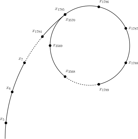
More importantly, such a function really does give a self-map of \(\mathbf Z_p\). That is, it has the following property: if \(x\equiv y\pmod p\), then \(f(x)\equiv f(y)\pmod p\).
Proof
If \(x\equiv y\pmod p\), then \(x^2+c\equiv y^2+c\pmod p\). Now \(f(x)=x^2+c-k_xN\), where \(k_x\) is an integer that depends on \(x\), and \(p\mid N\), so \(f(x)\equiv x^2+c\pmod p\) and therefore \(f(x)\equiv f(y)\pmod p\).
The sequence \(\{x_n\bmod p\}\) comes from iterating a pseudorandom self-map of \(\mathbf Z_p\), so it repeats within \(O(\sqrt p)\) expected time. As soon as we observe such a repetition \(x_i\equiv x_j\pmod p\), we get a nontrivial factor of \(N\) from \(\gcd(|x_i-x_j|,N)\). Since \(p\) is unknown, we cannot detect the repetition directly; a simple test is precisely that \(\gcd(|x_i-x_j|,N)\) is strictly greater than one.
The algorithm does not always succeed, because \(\gcd(|x_i-x_j|,N)\) may equal \(N\), that is, \(x_i\equiv x_j\pmod N\). In that case \(\{x_n\}\) happens to repeat at the very moment \(\{x_n\bmod p\}\) first repeats, and we get no nontrivial factor. Once \(\{x_n\}\) has started to cycle there is also no point in iterating further, since from then on it only repeats the cycle. The algorithm should report that the factorization has failed, and we have to factor again with a different \(c\) in \(f(x)\).
By the analysis above, in theory any function \(f(x)\) that satisfies \(\forall x \equiv y \pmod p, f(x) \equiv f(y) \pmod p\) and is reasonably pseudorandom (certain polynomial functions, for example) can be used here. In practice \(f(x)=x^2+c\ (c\neq 0,-2)\) is the main choice.2
Implementation
The algorithm we implement has to decide quickly, during the iteration, whether \(\{x_n\bmod p\}\) has already repeated. If we view \(f\) as the edges of a directed graph whose vertices are the elements of \(\mathbf Z_p\), what we really have to implement is a cycle detection algorithm, except that the equality test becomes a test of whether \(\gcd(|x_i-x_j|,N)\) is greater than one.
Floyd's cycle detection
Suppose two people are racing, A fast and B slow. After some time A is sure to meet B, and when they meet, the total distance A has run minus the total distance B has run is a multiple of the cycle length.
Let \(a=f(0),b=f(f(0))\) and update \(a=f(a),b=f(f(b))\) at every step. It suffices to check during the updates whether \(a\) and \(b\) are equal: once they are, a cycle has appeared.
At every step we set \(d=\gcd(|x_i-x_j|,N)\) and check whether \(d\) satisfies \(1< d< N\); if it does, we return \(d\) right away. If \(d=N\), then \(\{x_i\}\) has already formed a cycle, and once it has there is no point in going on: return \(N\) itself, then change the random constant \(c\) and factor again.
Pollard's rho algorithm with Floyd's cycle detection
1 2 3 4 5 6 7 8 9 10 11 12 13 | |
1 2 3 4 5 6 7 8 9 10 11 12 13 14 15 16 | |
Brent's cycle detection
Floyd's cycle detection can in fact be improved by a constant factor. Brent's cycle detection increases \(k\) starting from \(k=1\). In round \(k\), A waits in place while B moves forward \(2^k\) steps. If B meets A along the way, a cycle has been found; otherwise A teleports to B's position and the next round begins.
It can be proved3 that the number of calls to \(f\) needed before the cycle is found this way is never larger than with Floyd's cycle detection. The tests in the original paper show that Brent's cycle detection takes \(24\%\) less time on average than Floyd's.
Doubling optimization
With either Floyd's or Brent's cycle detection, the number of iterations is \(O(\sqrt p)\). But computing a \(\gcd\) in every iteration to test for a cycle slows the algorithm down. Accumulating a product reduces the number of \(\gcd\) computations.
In short, if \(\gcd(a,N)>1\), then \(\gcd(ab\bmod N,N)=\gcd(ab,N)>1\) holds for every \(b\in\mathbf N_+\). In other words, if we find that \(\gcd(\prod |x_i-x_j| \bmod N,N)>1\), then some pair \((x_i,x_j)\) among them must satisfy \(\gcd(|x_i-x_j|,N)>1\). If the product becomes zero at some point, the factorization has failed: quit and return \(N\) itself.
If a \(\gcd\) is computed once every \(k\) pairs, the complexity drops to \(O(\sqrt p+k^{-1}\sqrt p\log N)\), where \(\log N\) is the cost of a single \(\gcd\) computation. When \(k\) and \(\log N\) are of roughly the same order of magnitude, this gives an expected complexity of \(O(\sqrt p)\). Most implementations choose \(k=127\).
Here is an implementation of Pollard's rho algorithm with Brent's cycle detection and the doubling optimization.
Implementation
1 2 3 4 5 6 7 8 9 10 11 12 13 14 15 16 17 18 19 20 21 | |
1 2 3 4 5 6 7 8 9 10 11 12 13 14 15 16 17 18 19 20 21 22 23 24 | |
Complexity
The expected number of iterations of Pollard's rho algorithm is \(O(\sqrt p)\), where \(p\) is the smallest prime factor of \(N\). Whether an implementation uses Floyd's or Brent's cycle detection, its expected complexity without the doubling optimization is \(O(\sqrt p\log N)\); with the doubling optimization it is approximately \(O(\sqrt p)\).
Note that the analysis above assumes a truly random self-map, whereas Pollard's rho algorithm actually uses a pseudorandom function. The algorithm therefore has no rigorous complexity analysis; in practice it usually runs fast.
Example: finding the largest prime factor of a number
Example: P4718 [Template] Pollard-Rho Algorithm
For a number \(n\), use the Miller–Rabin algorithm to test whether it is prime. If it is, return right away. Otherwise use Pollard's rho algorithm to find a factor \(p\) and divide \(p\) out of \(n\). Then factor \(n\) and \(p\) recursively, using Miller–Rabin to tell when a prime factor has been reached and updating max_factor with it; this yields the largest prime factor. The data in this problem is far too large for Floyd's cycle detection to be enough, so the doubling optimization is used here.
Implementation
1 2 3 4 5 6 7 8 9 10 11 12 13 14 15 16 17 18 19 20 21 22 23 24 25 26 27 28 29 30 31 32 33 34 35 36 37 38 39 40 41 42 43 44 45 46 47 48 49 50 51 52 53 54 55 56 57 58 59 60 61 62 63 64 65 66 67 68 69 70 71 72 73 74 75 76 77 78 79 80 81 82 83 84 85 86 87 88 89 90 91 92 93 94 95 96 97 | |
References and links
-
https://en.wikipedia.org/wiki/Birthday_problem#Reverse_problem ↩
-
Menezes, Alfred J.; van Oorschot, Paul C.; Vanstone, Scott A. (2001). Handbook of Applied Cryptography. Section 3.11 and 3.12. ↩
-
Brent, R. P. (1980), An improved Monte Carlo factorization algorithm, BIT Numerical Mathematics, 20(2): 176–184, doi:10.1007/BF01933190 ↩
This page is an unofficial English translation of the original OI Wiki page (revision 4ac1e09c), machine-translated by Claude Fable 5.2 on 2026-11-16. It has been modified from the original by translation and may contain errors. It is not endorsed by OI Wiki.
Found a translation problem? Report it on GitHub.
Authors of the original page: Great-designer, StudyingFather, Xeonacid, Enter-tainer, 24OI-bot, kenlig, ksyx, Ir1d, iamtwz, Bubbleioa, SaisycJiang, Backl1ght, Menci, CCXXXI, shuzhouliu, TianKong-y, Tiphereth-A, 383494, GoodCoder666, wchyin, megakite, shawlleyw, c-forrest, Watersail2005 (full contribution history)
All content on this page is provided under the terms of CC BY-SA 4.0 and SATA; additional terms may apply.