Virtual Tree
Introduction
[SDOI2011] War of Attrition
In a war, the battlefield consists of \(n\) islands and \(n-1\) bridges, and it is guaranteed that exactly one path joins any two islands. Our army has found out that the enemy headquarters is on island \(1\) and that the enemy no longer has enough energy to keep fighting: victory is in sight. It is known that \(k\) other islands are rich in energy. To keep the enemy from getting hold of it, our army's task is to blow up some bridges so that the enemy cannot reach any energy-rich island. The bridges differ in material and structure, so blowing up different bridges has different costs, and our army wants to reach its goal at the minimum total cost.
The reconnaissance department has also found out that the enemy has a mysterious machine, which they can still use even after our army has cut off all the energy. The machine not only repairs every bridge our army has blown up, it also redistributes the resources at random (though it is guaranteed that no resources end up on island \(1\)). But the reconnaissance department has found out as well that the machine can be used only \(m\) times, so all we have to do is complete the task each time.
For all data, \(2\le n\le 2.5\times 10^5,1\le m\le 5\times 10^5,\sum k_i\le 5\times 10^5,1\le k_i\le n-1\).
Naive solution
For the problem above, if the tree has few nodes we can simply run a DP.
First, call the nodes selected in a query the key vertices.
Let \(Dp(i)\) be the minimum cost of disconnecting \(i\) from every key vertex in its subtree.
Let \(w(a,b)\) be the weight of the edge between \(a\) and \(b\).
Then enumerate the children \(v\) of \(i\):
- if \(v\) is not a key vertex: \(Dp(i)=Dp(i) + \min \{Dp(v),w(i,v)\}\);
- if \(v\) is a key vertex: \(Dp(i)=Dp(i) + w(i,v)\).
Good: this gives us an \(O(nq)\) program.
Sounds like fun.
Optimized solution
Many of the nodes are in fact useless. Take the tree below:
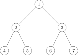
Suppose the key vertices we selected are:
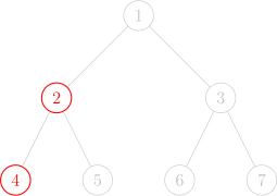
Only the two red nodes in the figure are key vertices; all the other nodes are non-key vertices.
For this problem, all we need is that the red nodes cannot reach node \(1\).
One look at the figure shows that the right subtree of node \(1\) (in general there may be several subtrees, but here there are only two, so let us call it that for now) contains no red node at all, so there is no need to run the DP on it.
By the constraints of the problem, the total number of red nodes (key vertices) is of the same order of magnitude as \(n\). In other words, the red nodes of a single query are very sparse in the whole tree, so it would be nice if the complexity depended on the total number of red nodes.
So we need to condense the information: condense one whole big tree into a small tree.
Virtual tree
This brings us to the concept of a virtual tree.
Let us first get a feeling for what a virtual tree looks like.
In the figures below, the red nodes are the key vertices we selected. The red and the black nodes are the nodes of the virtual tree, and the black edges are its edges.
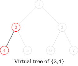
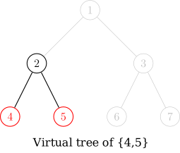
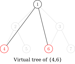
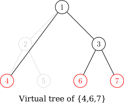
The LCA of any two key vertices also holds important information, so we have to keep these LCAs too. A virtual tree therefore need not consist of key vertices only.
Ancestor-descendant relations do not change in the virtual tree. (Nothing weird happens, such as \(a\) being an ancestor of \(b\) at first and ending up as a descendant of \(b\).)
But we cannot afford to enumerate the LCAs by brute force in \(O(k^2)\). A natural idea is to sort the key vertices by DFS order first, then take the LCA of every two adjacent key vertices (adjacent meaning that their indices in the sorted sequence differ by 1 in absolute value) and add it to the virtual tree.
The pressing question is how to construct the virtual tree.
Before proposing a method, let us settle one fact: as long as the ancestor-descendant relations are unchanged, we may add nodes to the virtual tree freely.
That is, if we felt like it, we could add every node of the original tree to the virtual tree without getting WA (though we would get TLE).
So for convenience we can start by adding node \(1\) to the virtual tree; this does not affect the answer.
First construction: sorting twice and adding edges by LCA
Several nodes may have one and the same LCA, so we must not add it to the virtual tree more than once.
A very intuitive method is:
- sort the key vertices by DFS order;
- make one pass, taking the LCA of every two adjacent key vertices and removing duplicates;
- then build the tree from the ancestor-descendant relations in the original tree.
In detail: go through the sequence of key vertices, take the LCA of every two adjacent entries, and add it to a sequence \(A\).
By the properties of the DFS order, the sequence \(A\) now contains every node of the virtual tree, though possibly more than once.
So we sort \(A\) in increasing DFS order and remove the duplicates.
Finally, for every two adjacent node indices \(x\) and \(y\) in the sequence \(A\), compute their LCA and connect \(\operatorname{LCA}(x,y)\) and \(y\). This completes the virtual tree.
Why does connecting \(\operatorname{LCA}(x,y)\) and \(y\) produce every edge exactly once?
Proof
If \(x\) is an ancestor of \(y\), we add the edge from \(x\) to \(y\) directly. The DFS order guarantees that \(x\) and \(y\) are adjacent in DFS order, so there is no key vertex on the path from \(x\) to \(y\).
If \(x\) is not an ancestor of \(y\), treat \(\operatorname{LCA}(x,y)\) as the ancestor of \(y\). By the previous case, there is no key vertex on the path from \(\operatorname{LCA}(x,y)\) to \(y\) either.
So connecting \(\operatorname{LCA}(x,y)\) and \(y\) misses no edge and repeats none.
What about the first node, which no node is connected to in this way: does that matter? No, because the first node must be the root of the tree. So the total number of edges is \(m-1\).
It takes at least two real vertices to conjure up one virtual vertex; add one root node, and the number of nodes in the virtual tree is twice the number of real vertices.
The time complexity is \(O(m\log n)\), where \(m\) is the number of key vertices and \(n\) is the total number of nodes.
Implementation
1 2 3 4 5 6 7 8 9 10 11 12 13 14 15 16 17 18 19 20 21 | |
This is in fact already enough to construct a virtual tree.
Second construction: with a monotonic stack
How do we construct a virtual tree with a monotonic stack?
First, let us be clear about the aim: the monotonic stack maintains one path of the virtual tree.
That is, two nodes adjacent in the stack are also adjacent in the virtual tree, and the stack is increasing from the bottom to the top (meaning that the nodes in the stack are in increasing DFS order). Put plainly, the parent of a node is the node just below it in the stack.
First push node \(1\) onto the stack.
Then add the key vertices in increasing DFS order.
If the LCA of the current node and the node on top of the stack is that top node, the two lie on one path, so just push the current node.
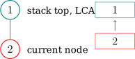
If the LCA of the current node and the top node is not the top node:
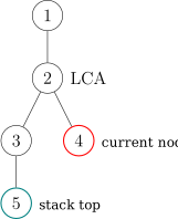
At this point the path maintained by the monotonic stack is:
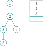
We need to turn it into:
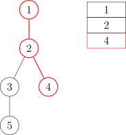
So we pop the nodes drawn with dashed lines. Before popping a node, do not forget to add an edge to its parent in the virtual tree.
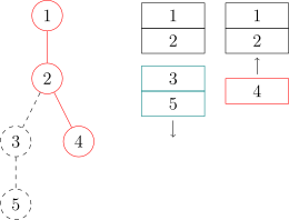
If the top of the stack after popping is not the LCA, push the LCA.
Then push the current node.
Here is a concrete example. Suppose we want to build the virtual tree of nodes 4, 6 and 7 in the tree below:
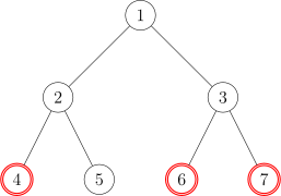
The steps are as follows:
- Sort the 3 key vertices \(6,4,7\) by DFS order to get the sequence \([4,6,7]\).
- Push \(1\).
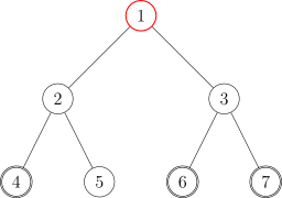
Red nodes are the nodes in the stack, and teal nodes are the nodes that have been popped from it.
- Take the first entry of the sequence as the current node: it is \(4\). The top element of the stack is \(1\). Compute the LCA of \(1\) and \(4\): \(LCA(1,4)=1\).
- Since \(LCA(1,4)=\) the top element, the two lie on one path of the virtual tree, so push the current node \(4\) directly. The stack is now \(4,1\).
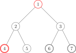
- Take the second entry of the sequence as the current node: it is \(6\). The top element of the stack is \(4\). Compute the LCA of \(6\) and \(4\): \(LCA(6,4)=1\).
- Since \(LCA(6,4)\neq\) the top element, enter the checking phase.
- Checking phase: the top node \(4\) comes after \(LCA(6,4)\) in DFS order, but the second-largest node (the one just below the top node), \(1\), has the same index in the DFS order as the LCA (and equal indices mean it is the same node). So the LCA is already in the stack. Add the edge \(1\to4\), that is, the edge from the LCA to the top element, and pop \(4\) from the stack.
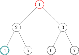
- The checking phase is over. Push \(6\); the stack is now \(6,1\).
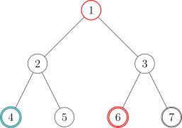
- Take the third entry of the sequence as the current node: it is \(7\). The top element of the stack is \(6\). Compute the LCA of \(7\) and \(6\): \(LCA(7,6)=3\).
- Since \(LCA(7,6)\neq\) the top element, enter the checking phase.
- Checking phase: the top node \(6\) comes after \(LCA(7,6)\) in DFS order, but the second-largest node (the one just below the top node), \(1\), comes before the LCA. So the LCA has never been pushed. Add the edge \(3\to6\), that is, the edge from the LCA to the top element. Pop \(6\) from the stack and push \(LCA(6,7)\).
- The checking phase is over. Push \(7\); the stack is now \(1,3,7\).
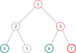
- All 3 nodes of the sequence have now been pushed, so leave the loop.
- The stack still holds 3 nodes: \(1,3,7\). They clearly lie on one path, so just add the edges \(1\to3\) and \(3\to7\).
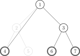
- The virtual tree is built!
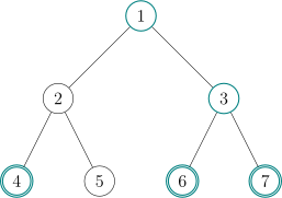
Now delete the nodes that were never pushed (the nodes that are not teal). The resulting virtual tree looks like this:
There are many details to get right. For instance, if the virtual tree is stored as an adjacency list, the adjacency list has to be cleared. Clearing the whole adjacency list is slow, so we clear the adjacency list of an element at the moment it is pushed for the first time.
The time complexity is again \(O(m\log n)\) (because of the sort), where \(m\) is the number of key vertices and \(n\) is the total number of nodes.
Implementation
The C++ code that builds the virtual tree looks roughly like this:
Implementation
1 2 3 4 5 6 7 8 9 10 11 12 13 14 15 16 17 18 19 20 21 22 23 24 25 26 27 28 29 30 31 32 33 | |
And now we know how to build a virtual tree!
For War of Attrition, just run the DP described at the very beginning on the virtual tree. In effect we have used the virtual tree to get rid of the useless non-key vertices! Again consider every child \(v\) of \(i\):
- if \(v\) is not a key vertex: \(Dp(i)=Dp(i) + \min \{Dp(v),w(i,v)\}\)
- if \(v\) is a key vertex: \(Dp(i)=Dp(i) + w(i,v)\)
And with that, the problem is easily solved.
Recommended practice problems
- [SDOI2011] War of Attrition
- [HEOI2014] Big Project
- CF613D Kingdom and its Cities
- [HNOI2014] World Tree
This page is an unofficial English translation of the original OI Wiki page (revision 3b4ab551), machine-translated by Claude Fable 5.2 on 2026-11-16. It has been modified from the original by translation and may contain errors. It is not endorsed by OI Wiki.
Found a translation problem? Report it on GitHub.
Authors of the original page: HeRaNO, Ir1d, konnyakuxzy, ksyx, Xeonacid, greyqz, sshwy, y-kx-b, yjl9903, 24OI-bot, tth37, ouuan, Chiechun, william-song-shy, Henry-ZHR, H-J-Granger, StudyingFather, Early0v0, Enter-tainer, HTensor, mcendu, iamtwz, Persdre, shuzhouliu, CoelacanthusHex, aofall, Marcythm, Tiphereth-A, SmallTualatin, szdytom, hyx1124, r-value, alphagocc, megakite, AxolotlXD666, shiftooo, tder6, GoodCoder666, lailai0916, sun2snow (full contribution history)
All content on this page is provided under the terms of CC BY-SA 4.0 and SATA; additional terms may apply.